5.4 mutually exclusive events

May 1, 2013Download as pptx, pdf

1 like2,459 views

Gary Ball

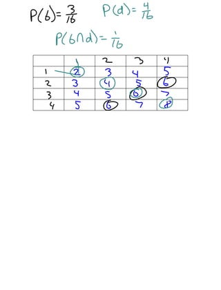
This document defines and provides examples of simple, compound, mutually exclusive and inclusive events. It explains that for mutually exclusive events, the probability of A or B equals the sum of the individual probabilities, while for inclusive events it equals the sum of the individual probabilities minus the probability they both occur. It then gives examples of calculating probabilities for various card draws and die rolls.

Lesson 8 conic sections - parabolaJean Leano

��

The document defines conic sections and describes parabolas. It provides specific objectives related to defining conic sections, identifying different types, describing parabolas, and converting between general and standard forms of parabola equations. It then gives details on the focus, directrix, vertex, latus rectum, and eccentricity of parabolas. Examples of problems involving finding parabola equations and properties from conditions are also provided.

Equation of the lineEdgardo Mata

��

1. The document discusses various forms of linear equations including general, two-point, intercept, point-slope, and slope-intercept forms. 2. It provides examples of writing equations in each form given specific information like two points, an x-intercept and y-intercept, a point and slope, or just a slope and y-intercept. 3. Guided practice problems are included for writing equations parallel or perpendicular to a given line.

Parabolaheiner gomez

��

The document discusses parabolas and their key properties: - A parabola is defined as the set of points equidistant from a fixed point (the focus) and a fixed line (the directrix). - The vertex is the point where the axis of symmetry intersects the parabola. The focus and directrix are a fixed distance (p) from the vertex. - The latus rectum is the line segment from the focus to the parabola, perpendicular to the axis of symmetry. Its length is determined by the equation of the parabola.

Adding and Subtracting Monomialsapacura

��

The document provides instructions on how to add and subtract monomials. It defines key terms like coefficient, base, exponent, degree of a monomial, degree of a polynomial, and like terms. It explains that to add monomials, you add the coefficients and keep the base, and to subtract monomials you subtract the coefficients and keep the base. Examples are given of simplifying expressions by combining like terms.

Chapter 5 Slope-Intercept FormIinternational Program School

��

This document provides a lesson on writing and graphing linear equations in slope-intercept form. It begins with examples of finding the slope and y-intercept of lines and writing the equation in the form y = mx + b. Then it shows how to graph lines from their equations in slope-intercept form. Applications include writing cost functions and finding values. A quiz reviews writing equations from slopes and points and graphing lines from their equations.

Graph of linear equationsanettebasco

��

This document discusses four methods for graphing linear equations on a coordinate plane: 1. Using any two points on the line. 2. Using the x-intercept and y-intercept. 3. Using the slope and y-intercept. 4. Using the slope and one known point. Examples are provided to illustrate each method. Graphing linear equations is important for visualizing relationships between variables in real-life situations.

12. Angle of Elevation & Depression.pptxBebeannBuar1

��

This document discusses angles of elevation and depression. It defines an angle of elevation as the angle formed between a horizontal line and the line of sight to an object located above the horizontal line. An angle of depression is defined as the angle formed between a horizontal line and the line of sight to an object located below the horizontal line. The document provides examples of solving problems involving angles of elevation and depression using trigonometric functions like tangent, sine, and the Pythagorean theorem. It emphasizes drawing a diagram, identifying if it is an angle of elevation or depression, and using the appropriate trigonometric ratio to solve for missing lengths.

11.3 slope of a lineGlenSchlee

��

This document discusses finding the slope of a line from two points or an equation. It provides the slope formula and explains how to calculate slope given two points on a line. It also discusses horizontal and vertical lines, which have slopes of 0 and undefined, respectively. The document shows how to find the slope of a line from its equation by solving for y and taking the coefficient of x. It concludes by explaining how to determine if two lines are parallel, perpendicular, or neither based on the equality or product of their slopes. Examples are provided to demonstrate these concepts.

nature of the roots and discriminantmaricel mas

��

This document provides guidance on identifying the nature of roots of quadratic equations. It begins by identifying the least mastered skill of identifying the nature of roots. It then reviews the standard form of a quadratic equation and the quadratic formula. The key concept of the discriminant is explained, which determines the number and type of roots. Examples are provided to show how to find the discriminant and use it to describe the nature of roots. Activities are included for students to practice rewriting equations in standard form, finding a, b, c values, calculating discriminants, and determining the nature of roots. An assessment card with example problems is provided to check understanding.

Ellipse.pptxJanuaryRegio

��

1. The document defines an ellipse and its key properties including its standard equation form. It discusses how an ellipse is a set of points where the sum of the distances to two fixed points (foci) is constant. 2. Parts of an ellipse like its vertices, covertices, axes, and directrices are defined. The standard equation of an ellipse centered at the origin is derived. 3. Examples are provided of determining the coordinates of foci, vertices, covertices, and directrices from equations. Problems involving finding equations or properties given certain conditions are also presented.

Introduction to Polynomial Functionskshoskey

��

This document provides an introduction to polynomial functions including definitions of key terms like monomial, polynomial, standard form, degree of terms and polynomials, classifying polynomials by number of terms and degree, examples of graphs of low-degree polynomials, and how to combine like terms. It defines a monomial as an expression with variables and numbers, a polynomial as a sum of terms with whole number exponents. Standard form writes polynomials in descending order of exponents. Degree is determined by highest exponent of terms or polynomial. Polynomials are classified by number of terms (monomial, binomial, trinomial, etc.) or degree (linear, quadratic, cubic, etc.). Examples show graphs changing shape with increasing degree. Combining like terms adds coefficients of

Factoring Difference of Two SquaresFree Math Powerpoints

��

equation of the line using two point formJessebelBautista

��

This document discusses using the two-point form to find the equation of a line given two points. It provides the two-point form equation, examples of using the form to find the slope and y-intercept of lines, and practice problems for determining the equation of lines passing through two points. The goal is to determine the equation in slope-intercept form using the two-point form equation and substituting the x- and y-coordinates of the two points.

Rational expressions pptDoreen Mhizha

��

5.1 expressions powerpointCristen Gillett

��

This document discusses expressions in algebra. It defines mathematical expressions and algebraic expressions, noting that algebraic expressions contain variables. It explains variables, coefficients, and constant terms. It provides examples of writing variable expressions from verbal phrases and vice versa. The document also discusses evaluating expressions by substituting values for variables and using order of operations. It includes practice problems for writing expressions, translating between verbal and algebraic forms, and evaluating expressions.

6 - NATURE OF THE ROOTS OF A QUADRATIC EQUATION USING DISCRIMINANT [Autosaved...bernadethvillanueva1

��

This document discusses using the discriminant of a quadratic equation (b^2 - 4ac) to characterize the nature of its roots. It defines the discriminant and explains that if the discriminant is equal to 0, the roots are real and equal. If the discriminant is positive and a perfect square, the roots are rational and unequal, and if positive but not a perfect square the roots are irrational and unequal. If the discriminant is negative, there are no real roots. Examples are provided to illustrate these concepts.

4 2 rules of radicalsmath123b

��

The document discusses rules for simplifying radical expressions. It states the square root and multiplication rules, which are that the square root of a squared term is the term itself, and that the square root of a product is the product of the square roots. Examples are provided to demonstrate applying these rules to simplify radical expressions by extracting square factors from the radicand. The division rule for radicals is also stated.

GRADE 10 ARITHMETIC.pptxDesireTSamillano

��

Equations of a Linesheisirenebkm

��

This document provides instruction on writing equations of lines using different forms: slope-intercept, point-slope, two-point, and intercept forms. Examples are given for writing equations of lines when given characteristics like slope, points, or intercepts. The last section presents an application example of using line equations to determine if two sets of bones found in an excavation site are parallel.

Introduction of Probabilityrey castro

��

This document defines key concepts in probability, including experiments, outcomes, sample spaces, events, unions and intersections of events, complements of events, mutually exclusive events, and the probability of independent and dependent events. It provides examples to illustrate these concepts, such as calculating the probability of drawing cards from a deck or marbles from a box. Formulas are given for calculating probabilities of unions, intersections, complements, mutually exclusive and inclusive events.

Circle lessonarvin gutierrez

��

This document discusses conic sections and circles. It defines conic sections as sections obtained when a plane cuts through a circular cone. It defines a circle as the set of all points equidistant from a fixed center point, where the fixed distance is called the radius. The document also mentions that Apollonius, a Greek mathematician, studied conic sections and gave them their names. He believed they should be studied for their mathematical beauty rather than practical applications.

Variable and Algebraic ExpressionsYelena Melnichenko

��

Algebraic expressions and equationsChristian Costa

��

This document defines key algebraic concepts such as variables, constants, expressions, terms, and polynomials. It explains that variables represent numbers with changing values, while constants have fixed values. Algebraic expressions combine variables and constants using operations. Polynomials are expressions made of one or more monomial terms, and can be classified by the number of terms. The document also covers degrees of monomials and polynomials, and provides examples of simplifying polynomials and determining their degrees.

Graphs of polynomial functionsCarlos Erepol

��

The document summarizes key characteristics of polynomial functions: 1) Polynomial functions produce smooth, continuous curves on their domains which are the set of real numbers. 2) The graph's x-intercepts, turning points, and absolute/relative maxima and minima are defined. 3) As the degree of a polynomial increases, so do the possible number of x-intercepts and turning points, up to the degree value. The leading coefficient and degree determine whether the graph rises or falls.

Distance between two pointslothomas

��

The document explains how to calculate the distance between two points using the distance formula. It shows that if points are horizontal or vertical, you can use their x- or y-coordinates alone, but otherwise you need to use the Pythagorean theorem to form a right triangle and find the hypotenuse. The distance formula is given as the square root of the sum of the squared differences between corresponding x- and y-coordinates of the two points. An example using points (3, -5) and (-1, 4) demonstrates applying the formula to find the distance between two points.

2.5.6 Perpendicular and Angle Bisectorssmiller5

��

The document outlines concepts related to perpendicular and angle bisectors, including their construction and applications in geometry. It explains the theorems related to these bisectors, such as the perpendicular bisector theorem and angle bisector theorem, along with their converses. Additionally, it defines the circumcenter and incenter of a triangle as key points derived from these bisectors.

Tangent lines PowerPointzackomack

��

This document discusses tangent lines. It defines a tangent line as a straight line that touches a curve at only one point. It explains that tangent lines are used to find the slope and instantaneous velocity or acceleration at a single point on a graph. The document contrasts tangent lines with secant lines, which touch a graph at two points, and notes that a vertical tangent line indicates a non-differentiable point with undefined slope. Examples of finding tangent lines are provided but refer to an external PowerPoint document.

4 3 Addition Rules for Probabilitymlong24

��

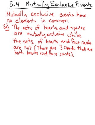
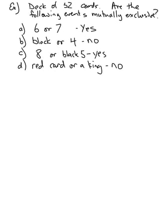
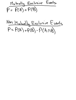
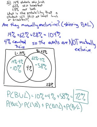
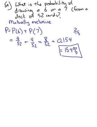
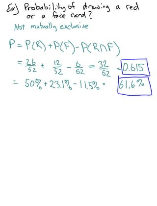
This document discusses the addition rules for probability of compound events. It defines mutually exclusive events as events that cannot occur at the same time, and explains that for mutually exclusive events A and B, the probability of A or B is equal to the probability of A plus the probability of B. For events that are not mutually exclusive, the probability of A or B is equal to the probability of A plus the probability of B minus the probability of A and B occurring together. Several examples are provided to illustrate calculating probabilities using these addition rules.

6.2 characteristics of polynomial functionsGary Ball

��

More Related Content

What's hot (20)

11.3 slope of a lineGlenSchlee

��

nature of the roots and discriminantmaricel mas

��

Ellipse.pptxJanuaryRegio

��

Introduction to Polynomial Functionskshoskey

��

Factoring Difference of Two SquaresFree Math Powerpoints

��

equation of the line using two point formJessebelBautista

��

Rational expressions pptDoreen Mhizha

��

5.1 expressions powerpointCristen Gillett

��

6 - NATURE OF THE ROOTS OF A QUADRATIC EQUATION USING DISCRIMINANT [Autosaved...bernadethvillanueva1

��

4 2 rules of radicalsmath123b

��

GRADE 10 ARITHMETIC.pptxDesireTSamillano

��

Equations of a Linesheisirenebkm

��

Introduction of Probabilityrey castro

��

Circle lessonarvin gutierrez

��

Variable and Algebraic ExpressionsYelena Melnichenko

��

Algebraic expressions and equationsChristian Costa

��

Graphs of polynomial functionsCarlos Erepol

��

Distance between two pointslothomas

��

2.5.6 Perpendicular and Angle Bisectorssmiller5

��

Tangent lines PowerPointzackomack

��

11.3 slope of a lineGlenSchlee

��

nature of the roots and discriminantmaricel mas

��

Ellipse.pptxJanuaryRegio

��

Introduction to Polynomial Functionskshoskey

��

Factoring Difference of Two SquaresFree Math Powerpoints

��

equation of the line using two point formJessebelBautista

��

Rational expressions pptDoreen Mhizha

��

5.1 expressions powerpointCristen Gillett

��

6 - NATURE OF THE ROOTS OF A QUADRATIC EQUATION USING DISCRIMINANT [Autosaved...bernadethvillanueva1

��

4 2 rules of radicalsmath123b

��

GRADE 10 ARITHMETIC.pptxDesireTSamillano

��

Equations of a Linesheisirenebkm

��

Introduction of Probabilityrey castro

��

Circle lessonarvin gutierrez

��

Variable and Algebraic ExpressionsYelena Melnichenko

��

Algebraic expressions and equationsChristian Costa

��

Graphs of polynomial functionsCarlos Erepol

��

Distance between two pointslothomas

��

2.5.6 Perpendicular and Angle Bisectorssmiller5

��

Tangent lines PowerPointzackomack

��

Viewers also liked (16)

4 3 Addition Rules for Probabilitymlong24

��

6.2 characteristics of polynomial functionsGary Ball

��

5.5 conditional probabiltyGary Ball

��

different kinds of probabilityMaria Romina Angustia

��

The document provides a history of the development of probability theory from its origins in the 16th century to modern applications. Some of the key contributors and advances mentioned include: - Cardan wrote one of the earliest works on probability in dice rolls and games of chance in 1550. - Pascal and Fermat laid the foundations of probability theory in correspondence solving gambling problems in 1654. - Graunt analyzed mortality data and made predictions, gaining access to the Royal Society of London. - Huygens published the first text on probability theory in 1657 introducing mathematical expectation. - Laplace's 1812 work outlined the evolution of probability theory and presented key theorems, establishing it as a rigorous

6.1 polynomial functionsGary Ball

��

5.3 probability using counting methodsGary Ball

��

Stat lesson 4.2 rules of computing probabilitypipamutuc

��

Here are the answers to the quiz questions: 1. a) The experiment is surveying teenagers about a newly developed soft drink and asking them to compare it with their favorite drink. b) One possible outcome is that a teenager prefers the new soft drink to their favorite drink. c) A possible event is that a teenager selected prefers Coke to the new soft drink. 2. A contingency table classifies observations according to two or more identifiable characteristics. It allows the computation of conditional probabilities. 3. The multiplication rule for independent events states that the probability of two independent events occurring together is equal to the product of their individual probabilities. So if A and B are independent, P(A and B) = P(

3.1 methods of divisionmath260

��

The document discusses polynomial division algorithms. It introduces long division and synthetic division as methods for dividing polynomials. Long division is analogous to dividing numbers, while synthetic division is simpler but only applies when dividing a polynomial by a monomial. The key points are: - Long division allows dividing any polynomial P(x) by any polynomial D(x) to obtain a quotient Q(x) and remainder R(x) such that P(x) = Q(x)D(x) + R(x) and the degree of R(x) is less than the degree of D(x). - Synthetic division is more efficient than long division when dividing a polynomial by a monomial of the form (

Independent and Dependent Eventsctybishop

��

This document discusses independent and dependent events and how to calculate probabilities of compound events. It defines probability as the likelihood of an event occurring. Compound events involve two or more simple events, and the probability is calculated by multiplying the probabilities of each individual event. Independent events do not influence each other, while dependent events are influenced by previous outcomes. The document provides examples comparing calculating probabilities of pulling beads from a bag with and without replacement.

Probability - Independent & Dependent EventsBitsy Griffin

��

Notes - Polynomial DivisionLori Rapp

��

1. Write the dividend and divisor with the divisor outside the long division bar. 2. Divide the first term of the dividend by the divisor and write the result above the division bar. 3. Multiply the divisor by the result and write the product below the terms of the dividend. 4. Subtract to find the remainder and bring down the next term to continue the process until there is no remainder. This document explains how to perform long division of polynomials using the same process as long division of numbers. It provides an example of performing long division step-by-step to divide a quadratic polynomial by a linear polynomial.

Long division, synthetic division, remainder theorem and factor theoremJohn Rome Aranas

��

This document summarizes four methods for working with polynomials: long division, synthetic division, the remainder theorem, and the factor theorem. It provides examples of using each method to divide the polynomial 4x^4 + 2x^3 + x + 5 by the divisor x + 2. Both long division and synthetic division yield a quotient of 4x^3 - 6x^2 + 12x - 23 and remainder of 51. The remainder theorem and factor theorem also verify this solution.

ProbabilityRushina Singhi

��

The document provides an overview of key probability concepts including: 1. Random experiments, sample spaces, events, and the classification of events as simple, mutually exclusive, independent, and exhaustive. 2. The three main approaches to defining probability: classical, relative frequency, and subjective. 3. Important probability theorems like the addition rule, multiplication rule, and Bayes' theorem. 4. How to calculate probabilities of events using these theorems, including examples of finding probabilities of independent, dependent, mutually exclusive, and conditional events.

PROBABILITY AND IT'S TYPES WITH RULESBhargavi Bhanu

��

This document discusses types of probability and provides definitions and examples of key probability concepts. It begins with an introduction to probability theory and its applications. The document then defines terms like random experiments, sample spaces, events, favorable events, mutually exclusive events, and independent events. It describes three approaches to measuring probability: classical, frequency, and axiomatic. It concludes with theorems of probability and references.

Basic Probability kaurab

��

This document discusses the concept of probability. It defines probability as a measure of how likely an event is to occur. Probabilities can be described using terms like certain, likely, unlikely, and impossible. Mathematically, probabilities are often expressed as fractions, with the numerator representing the number of possible outcomes for an event and the denominator representing the total number of possible outcomes. The document provides examples to illustrate concepts like independent and conditional probabilities, as well as complementary events and the gambler's fallacy.

Basic Concept Of Probabilityguest45a926

��

1. The document discusses basic concepts in probability and statistics, including sample spaces, events, probability distributions, and random variables. 2. Key concepts are explained such as independent and conditional probability, Bayes' theorem, and common probability distributions like the uniform and normal distributions. 3. Statistical analysis methods are introduced including how to estimate the mean and variance from samples from a distribution.

4 3 Addition Rules for Probabilitymlong24

��

6.2 characteristics of polynomial functionsGary Ball

��

5.5 conditional probabiltyGary Ball

��

different kinds of probabilityMaria Romina Angustia

��

6.1 polynomial functionsGary Ball

��

5.3 probability using counting methodsGary Ball

��

Stat lesson 4.2 rules of computing probabilitypipamutuc

��

3.1 methods of divisionmath260

��

Independent and Dependent Eventsctybishop

��

Probability - Independent & Dependent EventsBitsy Griffin

��

Notes - Polynomial DivisionLori Rapp

��

Long division, synthetic division, remainder theorem and factor theoremJohn Rome Aranas

��

ProbabilityRushina Singhi

��

PROBABILITY AND IT'S TYPES WITH RULESBhargavi Bhanu

��

Basic Probability kaurab

��

Basic Concept Of Probabilityguest45a926

��

More from Gary Ball (20)

4.6 combinationsGary Ball

��

This document discusses combinations and how to calculate them. It explains that a combination is an arrangement of objects from a group that considers order irrelevant. The document also provides the fundamental counting principle formula for combinations - nCr = n!/(r!(n-r)!) - and works through several examples of using the formula to calculate the number of possible combinations in different scenarios.

2.4 buy, rent, or leaseGary Ball

��

2.2 exploring credit card useGary Ball

��

7.3 substitution methodGary Ball

��

7.2 elimination methodGary Ball

��

4.1 fundamental counting principleGary Ball

��

4.1 slope of linear functionsGary Ball

��

4.1 slope of linear functionsGary Ball

��

4.1 slope of linear functionsGary Ball

��

3.1 sets and set notationGary Ball

��

3.4 applications of set theoryGary Ball

��

3.4 applications of set theoryGary Ball

��

3.3 intersection and unionGary Ball

��

3.1 sets and set notationGary Ball

��

3.1 sets and set notationGary Ball

��

2.3 problems involving creditGary Ball

��

2.4 even, odd, one to one, many to one functionsGary Ball

��

2.1 analyzing loansGary Ball

��

Multiplication tableGary Ball

��

Pa tournament drawGary Ball

��

4.6 combinationsGary Ball

��

2.4 buy, rent, or leaseGary Ball

��

2.2 exploring credit card useGary Ball

��

7.3 substitution methodGary Ball

��

7.2 elimination methodGary Ball

��

4.1 fundamental counting principleGary Ball

��

4.1 slope of linear functionsGary Ball

��

4.1 slope of linear functionsGary Ball

��

4.1 slope of linear functionsGary Ball

��

3.1 sets and set notationGary Ball

��

3.4 applications of set theoryGary Ball

��

3.4 applications of set theoryGary Ball

��

3.3 intersection and unionGary Ball

��

3.1 sets and set notationGary Ball

��

3.1 sets and set notationGary Ball

��

2.3 problems involving creditGary Ball

��

2.4 even, odd, one to one, many to one functionsGary Ball

��

2.1 analyzing loansGary Ball

��

Multiplication tableGary Ball

��

Pa tournament drawGary Ball

��

�ݺ�ߣ