ݺߣ

ݺߣShare a Scribd company logo
Chapter 52
Population Ecology
Population Dynamics
Survivorship Curves
Data in a life table can be represented
graphically by a survival curve.
Curve usually based on a standardized
population of 1000 individuals and the X-
axis scale is logarithmic.
Population dynamics
Survivorship curves can be classified into three
general types
Type I, Type II, and Type III
Figure 52.5
I
II
III
50 100
0
1
10
100
1,000
Percentage of maximum life span
Number
of
survivors
(log
scale)
Type I curve
Type I curve typical of animals that produce
few young but care for them well (e.g.
humans, elephants). Death rate low until
late in life where rate increases sharply as a
result of old age (wear and tear,
accumulation of cellular damage, cancer).
Type II curve
Type II curve has fairly steady death rate
throughout life (e.g. rodents).
Death is usually a result of chance processes
over which the organism has little control
(e.g. predation)
Type III curve
Type III curve typical of species that produce
large numbers of young which receive little or no
care (e.g. Oyster).
Survival of young is dependent on luck. Larvae
released into sea have only a small chance of
settling on a suitable substrate. Once settled
however, prospects of survival are much better
and a long life is possible.
Population growth
Occurs when birth rate exceeds death rate
(duh!)
Organisms have enormous potential to
increase their populations if not constrained
by mortality.
Any organism could swamp the planet in a
short time if it reproduced without restraint.
Per Capita Rate of Increase
If immigration and emigration are ignored,
a population’s growth rate (per capita
increase) equals the per capita birth rate
minus the per capita death rate
Equation for population growth is
ΔN/Δt = bN-dN
Where N = population size, b is per capita
birth rate and d is per capita death rate.
ΔN/Δt is change in population N over a
small time period t.
The per capita rate of population increase is
symbolized by r.
r = b-d.
r indicates whether a population is growing
(r >0) or declining (r<0).
Ecologists express instantaneous population
growth using calculus.
Zero population growth occurs when the
birth rate equals the death rate r = 0.
The population growth equation can be
expressed as dN
dt
 rN
Exponential population growth
(EPG)
Describes population growth in an
idealized, unlimited environment.
During EPG the rate of reproduction is at its
maximum.
The equation for exponential population
growth is
dN
dt
 rmaxN
The J-shaped curve of exponential growth
Is characteristic of some populations that are
rebounding
1900 1920 1940 1960 1980
Year
0
2,000
4,000
6,000
8,000
Elephant
population
Logistic Population Growth
Exponential growth cannot be sustained for
long in any population.
A more realistic population model limits
growth by incorporating carrying capacity.
Carrying capacity (K) is the maximum
population size the environment can support
The Logistic Growth Model
In the logistic population growth model the
per capita rate of increase declines as
carrying capacity is approached.
We construct the logistic model by starting
with the exponential model and adding an
expression that reduces the per capita rate of
increase as N increases
The logistic growth equation includes K, the
carrying capacity (number of organisms
environment can support)
As population size (N) increases, the equation ((K-N)/K)
becomes smaller which slows the population’s growth
rate.
Population dynamics
Logistic model produces a sigmoid (S-shaped) population
growth curve.
Logistic model predicts different per capita growth
rates for populations at low and high density. At
low density population growth rate driven
primarily by r the rate at which offspring can be
produced. At low density population grows
rapidly.
At high population density population growth is
much slower as density effects exert their effect.
800
600
400
200
0
Time (days)
0 5 10 15
(a) A Paramecium population in the lab.
The growth of Paramecium aurelia in
small cultures (black dots) closely
approximates logistic growth (red curve)
if the experimenter maintains a constant
environment.
1,000
Number
of
Paramecium/ml
The Logistic Model and Real
Populations
The growth of laboratory populations of
paramecia fits an S-shaped curve
Some populations overshoot K before settling down
to a relatively stable density
Figure 52.13b
180
150
0
120
90
60
30
Time (days)
0 160
140
120
80 100
60
40
20
Number
of
Daphnia/50
ml
(b) A Daphnia population in the lab. The growth of a population of Daphnia in a
small laboratory culture (black dots) does not correspond well to the logistic
model (red curve). This population overshoots the carrying capacity of its artificial
environment and then settles down to an approximately stable population size.
Some populations fluctuate greatly around K.
0
80
60
40
20
1975 1980 1985 1990 1995 2000
Time (years)
Number
of
females
(c) A song sparrow population in its natural habitat. The population of
female song sparrows nesting on Mandarte Island, British Columbia, is
periodically reduced by severe winter weather, and population growth is
not well described by the logistic model.
K-selection, or density-dependent selection
Selects for life history traits that are sensitive
to population density
r-selection, or density-independent selection
Selects for life history traits that maximize
reproduction
The concepts of K-selection and r-selection
have been criticized by ecologists as
oversimplifications.
Most organisms exhibit intermediate traits
or can adjust their behavior to different
conditions.

More Related Content

Similar to Population dynamics (20)

PPT
the population ecology 53_lecture_presentation_0.ppt
khalidmr1830
PPTX
8.4 effect of density of population.pptx
guggsds4
PPT
Population ecologyy
megha gupta
PPT
Population ecologyy
megha gupta
PPT
Chapter52
uv5
PDF
populationdynamicspresentation-130313073741-phpapp02.pdf
KifleLentiro1
PDF
Population ecology
MANSIMORE6
PPT
Unit2 Ecology Ib Populations Ppt2003
tnewberry
PPT
Population dynamics
kelliotluvsscience
PPT
Population dynamics
kelliotluvsscience
PPTX
Population growth
HARINATHA REDDY ASWARTHAGARI
PPTX
UNIT 2.pptxvvghhhhhhhhhjjjggffffghhjkkkkbvcddddd
uaddisababa
PPTX
Exponential and Logistics Growth Curve - Environmental Science
Nayan Dagliya
PPT
07 pop bio
dompiazza
PPTX
POPULATION AND BASIC POPULATION CHARACTERS.pptx
SherazSwati1
PPTX
14 (2013).pptx
NJJAISWALPC
PPT
Population-Ecology-shortenHsuwjwhwbushwhwhh.ppt
NathanielUba1
PPTX
Population ecology intro
Maria Donohue
PPT
Evol populations
Karl Pointer
PPTX
Environmental Science-4.pptx
Gavin Malala
the population ecology 53_lecture_presentation_0.ppt
khalidmr1830
8.4 effect of density of population.pptx
guggsds4
Population ecologyy
megha gupta
Population ecologyy
megha gupta
Chapter52
uv5
populationdynamicspresentation-130313073741-phpapp02.pdf
KifleLentiro1
Population ecology
MANSIMORE6
Unit2 Ecology Ib Populations Ppt2003
tnewberry
Population dynamics
kelliotluvsscience
Population dynamics
kelliotluvsscience
UNIT 2.pptxvvghhhhhhhhhjjjggffffghhjkkkkbvcddddd
uaddisababa
Exponential and Logistics Growth Curve - Environmental Science
Nayan Dagliya
07 pop bio
dompiazza
POPULATION AND BASIC POPULATION CHARACTERS.pptx
SherazSwati1
14 (2013).pptx
NJJAISWALPC
Population-Ecology-shortenHsuwjwhwbushwhwhh.ppt
NathanielUba1
Population ecology intro
Maria Donohue
Evol populations
Karl Pointer
Environmental Science-4.pptx
Gavin Malala

Recently uploaded (20)

PDF
Lesson 1 : Science and the Art of Geography Ecosystem
marvinnbustamante1
PPTX
How to Setup Automatic Reordering Rule in Odoo 18 Inventory
Celine George
PPTX
How to Create & Manage Stages in Odoo 18 Helpdesk
Celine George
PDF
TechSoup Microsoft Copilot Nonprofit Use Cases and Live Demo - 2025.06.25.pdf
TechSoup
PPTX
PLANNING A HOSPITAL AND NURSING UNIT.pptx
PRADEEP ABOTHU
PPTX
Ward Management: Patient Care, Personnel, Equipment, and Environment.pptx
PRADEEP ABOTHU
PDF
Lean IP - Lecture by Dr Oliver Baldus at the MIPLM 2025
MIPLM
PPTX
The Gift of the Magi by O Henry-A Story of True Love, Sacrifice, and Selfless...
Beena E S
PDF
The Power of Compound Interest (Stanford Initiative for Financial Decision-Ma...
Stanford IFDM
PDF
Andreas Schleicher_Teaching Compass_Education 2040.pdf
EduSkills OECD
PPTX
MATH 8 QUARTER 1 WEEK 1 LESSON 2 PRESENTATION
JohnGuillerNestalBah1
PDF
Free eBook ~100 Common English Proverbs (ebook) pdf.pdf
OH TEIK BIN
PPTX
ENGLISH 8 REVISED K-12 CURRICULUM QUARTER 1 WEEK 1
LeomarrYsraelArzadon
PPTX
How to Manage Wins & Losses in Odoo 18 CRM
Celine George
PPTX
Aerobic and Anaerobic respiration and CPR.pptx
Olivier Rochester
PPTX
Parsing HTML read and write operations and OS Module.pptx
Ramakrishna Reddy Bijjam
PPTX
Life and Career Skills Lesson 2.pptxProtective and Risk Factors of Late Adole...
ryangabrielcatalon40
PDF
IMPORTANT GUIDELINES FOR M.Sc.ZOOLOGY DISSERTATION
raviralanaresh2
PPTX
PLANNING FOR EMERGENCY AND DISASTER MANAGEMENT ppt.pptx
PRADEEP ABOTHU
PPTX
Marketing Management PPT Unit 1 and Unit 2.pptx
Sri Ramakrishna College of Arts and science
Lesson 1 : Science and the Art of Geography Ecosystem
marvinnbustamante1
How to Setup Automatic Reordering Rule in Odoo 18 Inventory
Celine George
How to Create & Manage Stages in Odoo 18 Helpdesk
Celine George
TechSoup Microsoft Copilot Nonprofit Use Cases and Live Demo - 2025.06.25.pdf
TechSoup
PLANNING A HOSPITAL AND NURSING UNIT.pptx
PRADEEP ABOTHU
Ward Management: Patient Care, Personnel, Equipment, and Environment.pptx
PRADEEP ABOTHU
Lean IP - Lecture by Dr Oliver Baldus at the MIPLM 2025
MIPLM
The Gift of the Magi by O Henry-A Story of True Love, Sacrifice, and Selfless...
Beena E S
The Power of Compound Interest (Stanford Initiative for Financial Decision-Ma...
Stanford IFDM
Andreas Schleicher_Teaching Compass_Education 2040.pdf
EduSkills OECD
MATH 8 QUARTER 1 WEEK 1 LESSON 2 PRESENTATION
JohnGuillerNestalBah1
Free eBook ~100 Common English Proverbs (ebook) pdf.pdf
OH TEIK BIN
ENGLISH 8 REVISED K-12 CURRICULUM QUARTER 1 WEEK 1
LeomarrYsraelArzadon
How to Manage Wins & Losses in Odoo 18 CRM
Celine George
Aerobic and Anaerobic respiration and CPR.pptx
Olivier Rochester
Parsing HTML read and write operations and OS Module.pptx
Ramakrishna Reddy Bijjam
Life and Career Skills Lesson 2.pptxProtective and Risk Factors of Late Adole...
ryangabrielcatalon40
IMPORTANT GUIDELINES FOR M.Sc.ZOOLOGY DISSERTATION
raviralanaresh2
PLANNING FOR EMERGENCY AND DISASTER MANAGEMENT ppt.pptx
PRADEEP ABOTHU
Marketing Management PPT Unit 1 and Unit 2.pptx
Sri Ramakrishna College of Arts and science
Ad

Population dynamics

  • 2. Survivorship Curves Data in a life table can be represented graphically by a survival curve. Curve usually based on a standardized population of 1000 individuals and the X- axis scale is logarithmic.
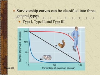
  • 4. Survivorship curves can be classified into three general types Type I, Type II, and Type III Figure 52.5 I II III 50 100 0 1 10 100 1,000 Percentage of maximum life span Number of survivors (log scale)
  • 5. Type I curve Type I curve typical of animals that produce few young but care for them well (e.g. humans, elephants). Death rate low until late in life where rate increases sharply as a result of old age (wear and tear, accumulation of cellular damage, cancer).
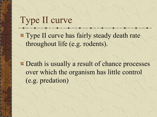
  • 6. Type II curve Type II curve has fairly steady death rate throughout life (e.g. rodents). Death is usually a result of chance processes over which the organism has little control (e.g. predation)
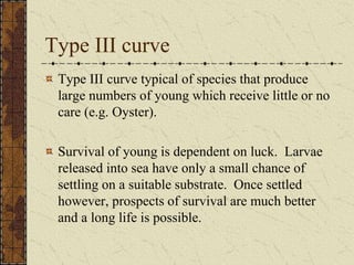
  • 7. Type III curve Type III curve typical of species that produce large numbers of young which receive little or no care (e.g. Oyster). Survival of young is dependent on luck. Larvae released into sea have only a small chance of settling on a suitable substrate. Once settled however, prospects of survival are much better and a long life is possible.
  • 8. Population growth Occurs when birth rate exceeds death rate (duh!) Organisms have enormous potential to increase their populations if not constrained by mortality. Any organism could swamp the planet in a short time if it reproduced without restraint.
  • 9. Per Capita Rate of Increase If immigration and emigration are ignored, a population’s growth rate (per capita increase) equals the per capita birth rate minus the per capita death rate
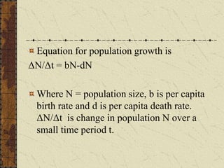
  • 10. Equation for population growth is ΔN/Δt = bN-dN Where N = population size, b is per capita birth rate and d is per capita death rate. ΔN/Δt is change in population N over a small time period t.
  • 11. The per capita rate of population increase is symbolized by r. r = b-d. r indicates whether a population is growing (r >0) or declining (r<0).
  • 12. Ecologists express instantaneous population growth using calculus. Zero population growth occurs when the birth rate equals the death rate r = 0. The population growth equation can be expressed as dN dt  rN
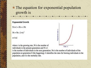
  • 13. Exponential population growth (EPG) Describes population growth in an idealized, unlimited environment. During EPG the rate of reproduction is at its maximum.
  • 14. The equation for exponential population growth is dN dt  rmaxN
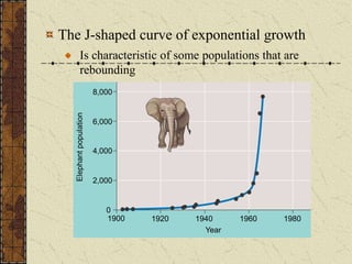
  • 15. The J-shaped curve of exponential growth Is characteristic of some populations that are rebounding 1900 1920 1940 1960 1980 Year 0 2,000 4,000 6,000 8,000 Elephant population
  • 16. Logistic Population Growth Exponential growth cannot be sustained for long in any population. A more realistic population model limits growth by incorporating carrying capacity. Carrying capacity (K) is the maximum population size the environment can support
  • 17. The Logistic Growth Model In the logistic population growth model the per capita rate of increase declines as carrying capacity is approached. We construct the logistic model by starting with the exponential model and adding an expression that reduces the per capita rate of increase as N increases
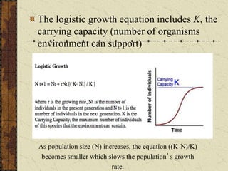
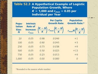
  • 18. The logistic growth equation includes K, the carrying capacity (number of organisms environment can support) As population size (N) increases, the equation ((K-N)/K) becomes smaller which slows the population’s growth rate.
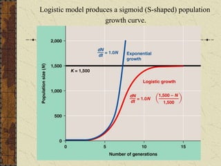
  • 20. Logistic model produces a sigmoid (S-shaped) population growth curve.
  • 21. Logistic model predicts different per capita growth rates for populations at low and high density. At low density population growth rate driven primarily by r the rate at which offspring can be produced. At low density population grows rapidly. At high population density population growth is much slower as density effects exert their effect.
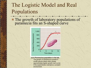
  • 22. 800 600 400 200 0 Time (days) 0 5 10 15 (a) A Paramecium population in the lab. The growth of Paramecium aurelia in small cultures (black dots) closely approximates logistic growth (red curve) if the experimenter maintains a constant environment. 1,000 Number of Paramecium/ml The Logistic Model and Real Populations The growth of laboratory populations of paramecia fits an S-shaped curve
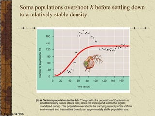
  • 23. Some populations overshoot K before settling down to a relatively stable density Figure 52.13b 180 150 0 120 90 60 30 Time (days) 0 160 140 120 80 100 60 40 20 Number of Daphnia/50 ml (b) A Daphnia population in the lab. The growth of a population of Daphnia in a small laboratory culture (black dots) does not correspond well to the logistic model (red curve). This population overshoots the carrying capacity of its artificial environment and then settles down to an approximately stable population size.
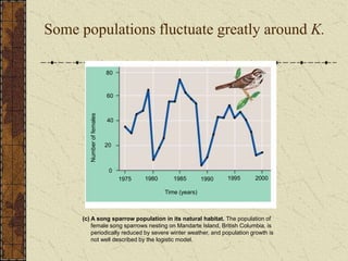
  • 24. Some populations fluctuate greatly around K. 0 80 60 40 20 1975 1980 1985 1990 1995 2000 Time (years) Number of females (c) A song sparrow population in its natural habitat. The population of female song sparrows nesting on Mandarte Island, British Columbia, is periodically reduced by severe winter weather, and population growth is not well described by the logistic model.
  • 25. K-selection, or density-dependent selection Selects for life history traits that are sensitive to population density r-selection, or density-independent selection Selects for life history traits that maximize reproduction
  • 26. The concepts of K-selection and r-selection have been criticized by ecologists as oversimplifications. Most organisms exhibit intermediate traits or can adjust their behavior to different conditions.