際際滷

際際滷Share a Scribd company logo
Wayland Free Library
e-Skills Shop
Presents
One Hour Study
Microsoft Excel
Course I
Skills Covered:
Revised: 3/2012
C. Petraitis
 WorkingwithTextinCells
 WorkingwithColumnsandRows
 FontGroup
 AlignmentGroup
e-Skills Shop Microsoft Excel
Course I
2
This document was produced by the Public Computing Center (PCC) at the Wayland Free
Library. The PCC was funded by a grant administered by the New York State Library, the lead
applicant for Broadbandexpress@yourlibrary grant. The State Library is a major unit within the
New York State Education Department, whose mission is to raise the knowledge, skill, and
opportunity for all the people in New York. The mission of the New York State Library, through
its Division of Library Development, is "to provide leadership and guidance for the planning and
coordinated development of library services and to serve as a reference and research library for
the people of the State."
The New York State Education Department (NYSED) was awarded $9.5 million in a matching
grant from the U.S. Department of Commerce National Telecommunications and Information
Administration (NTIA) to expand computer access in public libraries across New York State. The
funding is being provided through the American Reinvestment and Recovery Act (ARRA)
Broadband Technology Opportunities Program (BTOP).
Award Period: February 1, 2010 to January 31, 2013
e-Skills Shop Microsoft Excel
Course I
3
The One Hour Study courses are designed for you to create or learn a new computer skill in
under an hour. The courses are written in an easy to follow step-by-step manner with
illustrations to assist your learning. All you need is a computer to use, the manual for the skill
that you are going to learn, and a pen in case you want to make notes. As you progress through
this course, perform the instructions in each step and compare the results on the computer
monitor to the illustrations.
In this One Hour Study, you are going to learn the basic features of Excel. Feel free to write
notes in this manual, as it now belongs to you. If you have questions or need help, the e-Skills
Shop staff is available to assist you.
CELL BASICS
Excel uses columns and rows. Columns run vertically in
a spreadsheet and are labeled with capital letters. Rows
run horizontally in a spreadsheet and are labeled with
numbers. A cell is formed when a row and column
intersect. Each cell has an address or a name. The
address is the column letter followed by the row
number. The address also appears in the Name box.
STEP 1: To modify the contents of a cell, it must be
selected. To select it, click the cell. When it is selected,
the cells borders are black, and the column heading and
row heading are highlighted gold and the cells name
appears in the Name box as seen in Illustration 1. For
example, in Illustration 1, the cell C5 is selected. It is the intersection of column C and row 5.
Exercise:
1. Select cell A5. Notice the cells name in the Name box.
2. Select cell B13. Notice the cells name in the Name box.
3. Select cell G35. Notice the cells name in the Name box.
Column
Row
Name
box
Illustration 1
e-Skills Shop Microsoft Excel
Course I
4
Inserting Content
STEP 2: Click a cell to select it. When you type
text, notice the text appears in two locations: in
the cell and in the formula bar (Illustration 2).
STEP 3: There are several ways to move from cell
to cell. They are:
 Press Enter. The Enter key moves to the
cell below.
 The arrow keys. The arrow keys move to
the cell in the direction of the arrow.
 The Tab key. The Tab key selects the next cell to the right.
Exercise:
1. Type the following letters into the correct cell. When you have finished, you will have
the answer to the riddle below:
There is only one word in the English language with three
double letters in a row. What is it?
Answer: ____________________________________
Solution: The answer to the riddle is Bookkeeper.
Editing Content
STEP 4: There are two methods to edit the content in the cell:
Method 1: Double click the cell. You will see the insertion cursor in the cell. You are
able to edit the cell.
Method 2: Select the cell. Click the formula bar. The insertion cursor will be in the
formula bar, and you can edit the content in the formula bar.
Cell
Name
G4 H4 J4 B4 K4 C4 E4 D4 F4 I4
Letter E E E B R 0 K 0 K P
Formula Bar
Illustration 2
e-Skills Shop Microsoft Excel
Course I
5
Illustration 3
Deleting Content
STEP 5: Select the cell or cells.
STEP 6: Press the Delete key.
Exercise:
1. Change the word bookkeeper to bookkeeping.
2. Compare your work to Illustration 3.
3. Close Excel.
Exercise: Creating an Address Book
1. Start a new Excel workbook.
2. Save the workbook with the file name Address Book.
3. Enter the text into the cell indicated.
Cell Text Cell Text
A1 Last Name B1 First Name
C1 Company Name D1 Street Address
E1 State F1 City
G1 Zip H1 Home Phone
I1 Cell Phone J1 Birthday
4. Save and compare your work to Illustration 4.
Illustration 4
e-Skills Shop Microsoft Excel
Course I
6
MODIFYING COLUMNS AND ROWS
Column Width: There are four ways to adjust the width of
the columns.
Method 1:
STEP 7: Position your mouse over the column line in the
column heading. Your arrow will turn from a white cross
to a double headed black arrow.
STEP 8: Click and drag the column to the right to increase it or to the left to
decrease column width. Release the mouse.
Method 2:
STEP 9: Select the column(s) to modify by clicking the columns letter. This
selects the entire column (Illustration 5).
STEP 10: In the Cells group, click the Format command.
STEP 11: From the drop down menu, select Column Width (Illustration 6).
STEP 12: Enter a specific measurement in the Column Width dialog box
(Illustration 7). It is measured in characters.
STEP 13: Click OK.
Method 3:
STEP 14: Right click the column heading and select Column Width (Illustration 8).
STEP 15: Enter a specific measurement in the Column Width dialog box. It is
measured in characters.
STEP 16: Click OK.
Method 4:
STEP 17: Position your mouse over the right boundary of the column heading for
the column you want to adjust. Your pointer will turn from a white cross to a
Illustration 5
Illustration 6
Illustration 7
Illustration 8
e-Skills Shop Microsoft Excel
Course I
7
double headed black arrow. Double click. This will set the width to the size of the largest text.
Exercise: Use the Address Workbook.
1. Adjust the width of each column using the methods above.
2. Save and compare your work to Illustration 9.
Row Height: There are four methods to adjust the height of the rows.
Method 1:
STEP 18: Position your mouse between two rows. Your arrow will turn from a
white cross to a double headed black arrow.
STEP 19: Click and drag the row to the bottom of the screen to increase it or
to the top of the screen to decrease it. Release the mouse.
Method 2:
STEP 20: Select the column(s) to modify.
STEP 21: In the Cells group, click the Format command.
STEP 22: From the drop down menu, select Row Height (Illustration 10).
STEP 23: Enter a specific measurement in the Row Height dialog box. It is
measured in characters.
STEP 24: Click OK.
Method 3:
STEP 25: Right click the row heading and select Row Height (Illustration 11).
STEP 26: Enter a specific measurement in the Row Height dialog box. It is
measured in characters.
STEP 27: Click OK.
Illustration 9
Illustration 10
Illustration 11
e-Skills Shop Microsoft Excel
Course I
8
Method 4:
STEP 28: Position your mouse over the bottom boundary of the row heading for the row you
want to adjust. Your pointer will turn from a white cross to a double headed black arrow.
Double click. This will set the height to the size of the largest character to fit the text. (NOTE:
This method is used to remove extra space in the height of the cell)
Exercise: Use the Address Workbook.
1. Adjust the height of each rows 1-5.
2. Save and compare your work to Illustration 12.
Inserting Rows and Columns: Rows are always inserted above the current
location of the cursor. Columns are inserted to the left of the location of the
cursor. There are two ways to insert columns and rows:
Method 1: In the Cells group, click the Insert command (Illustration 13).
Method 2: Right click the column/row heading and select Insert (Illustration
14).
Exercise:
1. Insert a row above row 1.
2. In cell A1 type: Address Book
3. Insert a column to the left of Birthday. In cell J1 (the location of the new
column), type: E-Mail Address.
4. Adjust column width.
5. Save and compare your work to Illustration 15.
Illustration 13
Illustration 14
Illustration 12
Illustration 15
e-Skills Shop Microsoft Excel
Course I
9
Delete Rows and Columns:
Method 1: Select the column(s) or row(s) to delete. In the Cells group, click the
Delete command (Illustration 13).
Method 2: Select the column(s) or row(s) to delete. Right click and select
Delete (Illustration 16).
Exercise:
1. Delete column C, called Company.
2. Save and compare your work to Illustration 17.
FORMATTING CELLS
Font Group: The font group contains commands to change the
appearance of the text or numbers in the cells (Illustration 18).
STEP 29: Select the cell(s) to modify.
STEP 30: Select the command to use. Explanation of the commands
are below:
Change the Font: The Font command changes the appearance of the
text. Click the drop down arrow next to the Font command to view
choices (Illustration 18A).
Change the Font Size: The Font Size changes the size of the text. Click the drop down arrow
next to the Font size command to view the choices (Illustration 18B).
Grow Font: Increase the text size (Illustration 18C).
Shrink Font: Decreases the text size (Illustration 18D).
Bold: Bold darkens the text (Illustration 18E).
Illustration 16
Illustration 18
A B C D
E F G H I J
Illustration 17
e-Skills Shop Microsoft Excel
Course I
10
Illustration 19
Italics: Italics slants the text (Illustration 18F).
Underline: Underlines the text only (Illustration 18G).
Border: A border creates a border around the cell. Borders can be placed on any side of the
cell such as left, right, bottom, or top (Illustration 18H).
Fill Color: Changes the color of the cell (Illustration 18I).
Font Color: Changes the color of the text (Illustration 18J).
Exercise: Use the Address Workbook.
1. Select cells A2-J2 (HINT: Click the row to select the cells in that row).
2. Change the Font Style.
3. Change the Font Size.
4. Adjust the column and row size as needed.
5. Add a Border around the cells.
6. Select cell A1 and change the font.
7. Select row 2. Add a Fill Color.
8. Select row 4. Add a Fill Color.
9. Select row 6. Add a Fill Color.
10. Continue to explore the other commands in the Font group.
11. Save and compare your work to Illustration 19.
The Alignment Group: The Alignment Group
contains commands to change the location of the
text within the cell (Illustration 20).
Cell Alignment: Alignment is how text appears in
relationship to the margins. By default, text is
A
B
C
D E
F
Illustration 20
e-Skills Shop Microsoft Excel
Course I
11
bottom aligned at the left margin. Vertical and horizontal alignment can be used at the same
time (Illustration 20A).
 Vertical Alignment:
o Top Align: Align text to the top of the cell.
o Middle Align: Align text to the middle of the cell.
o Bottom Align: Align text to the bottom of the cell
 Horizontal Alignment:
o Align Text Left: Aligns text to the left of the cell.
o Center: Centers the text in the cell.
o Align Text Right: Aligns text to the right of the cell.
Wrap Text: Allows multi-lined text in a cell instead of text spread across a wide cell (Illustration
20B).
Merge and Center: Joins the selected cells into one large cell and centering the content
(Illustration 20C).
Decrease Indent: Decrease the margin between the border and the text in the cell (Illustration
20D).
Increase Indent: Increase the margin between the border and the text in the cell (Illustration
20E).
Orientation: Rotate text to a diagonal or vertical orientation (Illustration 20F).
Exercise: Use the Address Workbook.
1. Increase row 2s height.
2. Select row 2 and change the alignment of the text.
3. Decrease column C so the text is only partially visible.
4. With Column C selected, use the Wrap Text command to make all the text visible.
5. Select cells A1-J1.
6. Merge and Center the cells.
7. Continue to explore the commands in the Alignment group.
e-Skills Shop Microsoft Excel
Course I
12 Illustration 22
8. Save and compare your work to illustration 21.
COURSE REVIEW
 Edit cell content in the formula bar or by double clicking on the cell.
 Modify columns and rows by adjusting the columns in the heading, using the Format
command from the ribbon, right clicking on the heading, or double clicking over the
right/bottom boundary.
 Edit text by using the commands in the Font group.
TEST YOUR KNOWLEDGE
Exercise: Grocery List
1. Type the following text into the cell indicated:
Cell Text Cell Text
A1 Grocery List B3 Produce
D3 Natural/Organic F3 Meats & Seafood
B13 Health& Beauty D13 Cleaning&Household
F13 Condiments B23 Pasta
D23 Baking F23 Cereal & Snacks
Illustration 21
e-Skills Shop Microsoft Excel
Course I
13
B33 Dairy D33 Frozen
F33 Other
2. Select cell A1. Increase the font size and change the font style.
3. Select cells A1-F2. Merge and Center.
4. Change the font size and style of remaining text.
5. Resize columns and rows referring to Illustration 22 as a guide.
6. Wrap text if needed.
7. Change the alignment.
8. Use the Fill Color command.
9. Add borders.
10. Save and compare your work to Illustration 22.
Exercise: Gift Shopping List
1. Type the following text into the cell indicated:
Cell Text Cell Text
A1 Gift Shopping List F1 2012
B3 Christmas F3 Birthday
B4 Gift Ideas C4 Store Name or URL
D4 List Price E4 Purchase Price
F4 Gift Ideas G4 Store Name or URL
H4 List Price I4 Purchase Price
A5 Spouse A6 Mom
A7 Dad A8 Brother
A9 Sister A10 Friend
2. Select cell A1. Increase the font size and change the font style.
3. Select cells B3-E3. Merge and Center.
e-Skills Shop Microsoft Excel
Course I
14
4. Select cells F3-I3. Merge and Center.
5. Change the font size and style of remaining text.
6. Resize columns and rows.
7. Wrap text if needed.
8. Change the alignment.
9. Use the Fill Color command.
10. Add borders.
11. Type the following text into the cell indicated:
Cell Text
B5 I-Pod Touch
C5 Apple
D5 $200
B6 Crochet Blanket
C6 JoAnn Fabrics
D6 $30
B7 Gift Card
C7 Tractor Supply
D7 $40.00
B8 Harry Potter Box Set
C8 Amazon.com
D8 $43.76
e-Skills Shop Microsoft Excel
Course I
15
12. Save and compare your work to Illustration 23.
FURTHER READINGS
Library Books
Microsoft Office for the Older and Wiser Publisher by Sean McManus (2011) 005.5 MCM
Microsoft Excel 2010: Step by Step by Curtis Frye (2010) 005.54 C948
Office 2010 Simplified by Kate Shoup (2010) 005.5 SHO
Websites
GCF Learn Online (http://www.gcflearnfree.org/)
For further explanations of formulas, please watch the video from GCF LearnFree.org
(http://www.gcflearnfree.org/excel2010/6.2).
Microsoft Help and How To (office.microsoft.com/en-us/word-help/)
Illustration 23
Ad

Recommended

Whatsapp survery report
Karan Kukreja
MS Excel 2010 training module
Aijaz Ali Mooro
Libre Office Calc Lesson 5: Working with Data
Smart Chicago Collaborative
Chapter.06
Chapter.06
jdswitzer
MS Excel 2010 tutorial 2
Khalfan Alshuaili
Libre office calc
Libre office calc
Miguel Angel Romero Ochoa
Excel basics for everyday use
Kevin McLogan
Libre Office Calc Lesson 2: Formatting and Charts
Smart Chicago Collaborative
Excel
Excel
arbiesani
Microsoft Excel Presentation
Ram Bhandari
Libre Office Calc Lesson 4: Understanding Functions
Smart Chicago Collaborative
Excel for beginners class 1
Carlstadt Public Library
Excel training
Excel training
Alexandru Gologan
10 INTERSTING TRICKS FOR EXCEL
rahul kumar
Microsoft Excel Advanced Features
AkashMeghwar2
get_more_from_excel
get_more_from_excel
Kevin Hoult
Excel Tutorial
Excel Tutorial
Jayson Patalinghug
How to use a spreadsheet
Swarnima Tiwari
Excel Tutorials - Finding & Removing the Duplicate Values
Merve Nur Ta
Excel for beginners class 2
Carlstadt Public Library
Excel for kids
Excel for kids
Queens Library
Dash board
Dash board
Omar Farooq
MS Excel
MS Excel
Abdulbasit Hassan
Microsoft Excel 2007 Tutorial
Kereen Tatham
microsoft ecexl
microsoft ecexl
elfiSahara2
Excel Powerpoint class with video
Rich Johnson
Open Office Calc : Lesson 05
thinkict
W5_MSEXCEL.pdf
W5_MSEXCEL.pdf
ExtremelyDarkness2
Microsoft excel part 1
Hoboken Public Library
Unit 4 ms excel of class 8
Geethu Bijesh

More Related Content

What's hot (19)

Excel
Excel
arbiesani
Microsoft Excel Presentation
Ram Bhandari
Libre Office Calc Lesson 4: Understanding Functions
Smart Chicago Collaborative
Excel for beginners class 1
Carlstadt Public Library
Excel training
Excel training
Alexandru Gologan
10 INTERSTING TRICKS FOR EXCEL
rahul kumar
Microsoft Excel Advanced Features
AkashMeghwar2
get_more_from_excel
get_more_from_excel
Kevin Hoult
Excel Tutorial
Excel Tutorial
Jayson Patalinghug
How to use a spreadsheet
Swarnima Tiwari
Excel Tutorials - Finding & Removing the Duplicate Values
Merve Nur Ta
Excel for beginners class 2
Carlstadt Public Library
Excel for kids
Excel for kids
Queens Library
Dash board
Dash board
Omar Farooq
MS Excel
MS Excel
Abdulbasit Hassan
Microsoft Excel 2007 Tutorial
Kereen Tatham
microsoft ecexl
microsoft ecexl
elfiSahara2
Excel Powerpoint class with video
Rich Johnson
Open Office Calc : Lesson 05
thinkict
Microsoft Excel Presentation
Ram Bhandari
Libre Office Calc Lesson 4: Understanding Functions
Smart Chicago Collaborative
10 INTERSTING TRICKS FOR EXCEL
rahul kumar
Microsoft Excel Advanced Features
AkashMeghwar2
get_more_from_excel
get_more_from_excel
Kevin Hoult
How to use a spreadsheet
Swarnima Tiwari
Excel Tutorials - Finding & Removing the Duplicate Values
Merve Nur Ta
Microsoft Excel 2007 Tutorial
Kereen Tatham
microsoft ecexl
microsoft ecexl
elfiSahara2
Excel Powerpoint class with video
Rich Johnson
Open Office Calc : Lesson 05
thinkict

Similar to Microsoft excel 2010 course i (20)

W5_MSEXCEL.pdf
W5_MSEXCEL.pdf
ExtremelyDarkness2
Microsoft excel part 1
Hoboken Public Library
Unit 4 ms excel of class 8
Geethu Bijesh
Microsoft 2007 Basics
Julie Van Noy
Excel formulas tf-jul1605
Shaikh 愆悽 Kalim 擧
Excel training basic
TimesRide
MS EXCEL.ppt
MS EXCEL.ppt
DondonGoles
Excel PPTs.pptx
Excel PPTs.pptx
Rajneesh501415
Excel-Formulas.8735609.powerpoint.pptx
CheeneeRivera
EXCEL
EXCEL
Nagarajan murthy
Introduction to Microsoft EXCEL and uses.pptx
DondonGoles
Introduction to Microsoft - EXCEL and uses.ppt
DondonGoles
Introduction to micro soft Training ms Excel.ppt
dejene3
Training On Microsoft Excel
TimesRide
METHODS OF CUTTING COPYING HTML BASIC NOTES
Sitamarhi Institute of Technology
MS Excel and Visual Basic Applications.pptx
surekha1287
Microsoft excel power point presentation.pptx
sajidkhanindeedf
Microsoft excel tutorial (part i)
mariavarey
presentation on excel and word
Ma Hancy
5632010019,5632010020
5632010019,5632010020
ac5632010019
Unit 4 ms excel of class 8
Geethu Bijesh
Microsoft 2007 Basics
Julie Van Noy
Excel training basic
TimesRide
Excel-Formulas.8735609.powerpoint.pptx
CheeneeRivera
Introduction to Microsoft EXCEL and uses.pptx
DondonGoles
Introduction to Microsoft - EXCEL and uses.ppt
DondonGoles
Introduction to micro soft Training ms Excel.ppt
dejene3
Training On Microsoft Excel
TimesRide
MS Excel and Visual Basic Applications.pptx
surekha1287
Microsoft excel power point presentation.pptx
sajidkhanindeedf
Microsoft excel tutorial (part i)
mariavarey
presentation on excel and word
Ma Hancy
5632010019,5632010020
5632010019,5632010020
ac5632010019
Ad

Microsoft excel 2010 course i

  • 1. Wayland Free Library e-Skills Shop Presents One Hour Study Microsoft Excel Course I Skills Covered: Revised: 3/2012 C. Petraitis WorkingwithTextinCells WorkingwithColumnsandRows FontGroup AlignmentGroup
  • 2. e-Skills Shop Microsoft Excel Course I 2 This document was produced by the Public Computing Center (PCC) at the Wayland Free Library. The PCC was funded by a grant administered by the New York State Library, the lead applicant for Broadbandexpress@yourlibrary grant. The State Library is a major unit within the New York State Education Department, whose mission is to raise the knowledge, skill, and opportunity for all the people in New York. The mission of the New York State Library, through its Division of Library Development, is "to provide leadership and guidance for the planning and coordinated development of library services and to serve as a reference and research library for the people of the State." The New York State Education Department (NYSED) was awarded $9.5 million in a matching grant from the U.S. Department of Commerce National Telecommunications and Information Administration (NTIA) to expand computer access in public libraries across New York State. The funding is being provided through the American Reinvestment and Recovery Act (ARRA) Broadband Technology Opportunities Program (BTOP). Award Period: February 1, 2010 to January 31, 2013
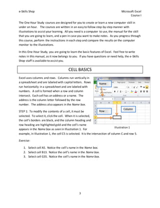
  • 3. e-Skills Shop Microsoft Excel Course I 3 The One Hour Study courses are designed for you to create or learn a new computer skill in under an hour. The courses are written in an easy to follow step-by-step manner with illustrations to assist your learning. All you need is a computer to use, the manual for the skill that you are going to learn, and a pen in case you want to make notes. As you progress through this course, perform the instructions in each step and compare the results on the computer monitor to the illustrations. In this One Hour Study, you are going to learn the basic features of Excel. Feel free to write notes in this manual, as it now belongs to you. If you have questions or need help, the e-Skills Shop staff is available to assist you. CELL BASICS Excel uses columns and rows. Columns run vertically in a spreadsheet and are labeled with capital letters. Rows run horizontally in a spreadsheet and are labeled with numbers. A cell is formed when a row and column intersect. Each cell has an address or a name. The address is the column letter followed by the row number. The address also appears in the Name box. STEP 1: To modify the contents of a cell, it must be selected. To select it, click the cell. When it is selected, the cells borders are black, and the column heading and row heading are highlighted gold and the cells name appears in the Name box as seen in Illustration 1. For example, in Illustration 1, the cell C5 is selected. It is the intersection of column C and row 5. Exercise: 1. Select cell A5. Notice the cells name in the Name box. 2. Select cell B13. Notice the cells name in the Name box. 3. Select cell G35. Notice the cells name in the Name box. Column Row Name box Illustration 1
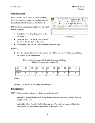
  • 4. e-Skills Shop Microsoft Excel Course I 4 Inserting Content STEP 2: Click a cell to select it. When you type text, notice the text appears in two locations: in the cell and in the formula bar (Illustration 2). STEP 3: There are several ways to move from cell to cell. They are: Press Enter. The Enter key moves to the cell below. The arrow keys. The arrow keys move to the cell in the direction of the arrow. The Tab key. The Tab key selects the next cell to the right. Exercise: 1. Type the following letters into the correct cell. When you have finished, you will have the answer to the riddle below: There is only one word in the English language with three double letters in a row. What is it? Answer: ____________________________________ Solution: The answer to the riddle is Bookkeeper. Editing Content STEP 4: There are two methods to edit the content in the cell: Method 1: Double click the cell. You will see the insertion cursor in the cell. You are able to edit the cell. Method 2: Select the cell. Click the formula bar. The insertion cursor will be in the formula bar, and you can edit the content in the formula bar. Cell Name G4 H4 J4 B4 K4 C4 E4 D4 F4 I4 Letter E E E B R 0 K 0 K P Formula Bar Illustration 2
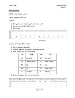
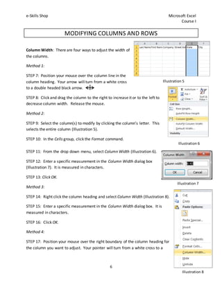
  • 5. e-Skills Shop Microsoft Excel Course I 5 Illustration 3 Deleting Content STEP 5: Select the cell or cells. STEP 6: Press the Delete key. Exercise: 1. Change the word bookkeeper to bookkeeping. 2. Compare your work to Illustration 3. 3. Close Excel. Exercise: Creating an Address Book 1. Start a new Excel workbook. 2. Save the workbook with the file name Address Book. 3. Enter the text into the cell indicated. Cell Text Cell Text A1 Last Name B1 First Name C1 Company Name D1 Street Address E1 State F1 City G1 Zip H1 Home Phone I1 Cell Phone J1 Birthday 4. Save and compare your work to Illustration 4. Illustration 4
  • 6. e-Skills Shop Microsoft Excel Course I 6 MODIFYING COLUMNS AND ROWS Column Width: There are four ways to adjust the width of the columns. Method 1: STEP 7: Position your mouse over the column line in the column heading. Your arrow will turn from a white cross to a double headed black arrow. STEP 8: Click and drag the column to the right to increase it or to the left to decrease column width. Release the mouse. Method 2: STEP 9: Select the column(s) to modify by clicking the columns letter. This selects the entire column (Illustration 5). STEP 10: In the Cells group, click the Format command. STEP 11: From the drop down menu, select Column Width (Illustration 6). STEP 12: Enter a specific measurement in the Column Width dialog box (Illustration 7). It is measured in characters. STEP 13: Click OK. Method 3: STEP 14: Right click the column heading and select Column Width (Illustration 8). STEP 15: Enter a specific measurement in the Column Width dialog box. It is measured in characters. STEP 16: Click OK. Method 4: STEP 17: Position your mouse over the right boundary of the column heading for the column you want to adjust. Your pointer will turn from a white cross to a Illustration 5 Illustration 6 Illustration 7 Illustration 8
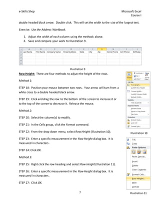
  • 7. e-Skills Shop Microsoft Excel Course I 7 double headed black arrow. Double click. This will set the width to the size of the largest text. Exercise: Use the Address Workbook. 1. Adjust the width of each column using the methods above. 2. Save and compare your work to Illustration 9. Row Height: There are four methods to adjust the height of the rows. Method 1: STEP 18: Position your mouse between two rows. Your arrow will turn from a white cross to a double headed black arrow. STEP 19: Click and drag the row to the bottom of the screen to increase it or to the top of the screen to decrease it. Release the mouse. Method 2: STEP 20: Select the column(s) to modify. STEP 21: In the Cells group, click the Format command. STEP 22: From the drop down menu, select Row Height (Illustration 10). STEP 23: Enter a specific measurement in the Row Height dialog box. It is measured in characters. STEP 24: Click OK. Method 3: STEP 25: Right click the row heading and select Row Height (Illustration 11). STEP 26: Enter a specific measurement in the Row Height dialog box. It is measured in characters. STEP 27: Click OK. Illustration 9 Illustration 10 Illustration 11
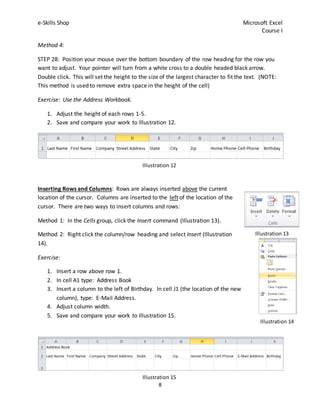
  • 8. e-Skills Shop Microsoft Excel Course I 8 Method 4: STEP 28: Position your mouse over the bottom boundary of the row heading for the row you want to adjust. Your pointer will turn from a white cross to a double headed black arrow. Double click. This will set the height to the size of the largest character to fit the text. (NOTE: This method is used to remove extra space in the height of the cell) Exercise: Use the Address Workbook. 1. Adjust the height of each rows 1-5. 2. Save and compare your work to Illustration 12. Inserting Rows and Columns: Rows are always inserted above the current location of the cursor. Columns are inserted to the left of the location of the cursor. There are two ways to insert columns and rows: Method 1: In the Cells group, click the Insert command (Illustration 13). Method 2: Right click the column/row heading and select Insert (Illustration 14). Exercise: 1. Insert a row above row 1. 2. In cell A1 type: Address Book 3. Insert a column to the left of Birthday. In cell J1 (the location of the new column), type: E-Mail Address. 4. Adjust column width. 5. Save and compare your work to Illustration 15. Illustration 13 Illustration 14 Illustration 12 Illustration 15
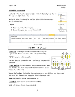
  • 9. e-Skills Shop Microsoft Excel Course I 9 Delete Rows and Columns: Method 1: Select the column(s) or row(s) to delete. In the Cells group, click the Delete command (Illustration 13). Method 2: Select the column(s) or row(s) to delete. Right click and select Delete (Illustration 16). Exercise: 1. Delete column C, called Company. 2. Save and compare your work to Illustration 17. FORMATTING CELLS Font Group: The font group contains commands to change the appearance of the text or numbers in the cells (Illustration 18). STEP 29: Select the cell(s) to modify. STEP 30: Select the command to use. Explanation of the commands are below: Change the Font: The Font command changes the appearance of the text. Click the drop down arrow next to the Font command to view choices (Illustration 18A). Change the Font Size: The Font Size changes the size of the text. Click the drop down arrow next to the Font size command to view the choices (Illustration 18B). Grow Font: Increase the text size (Illustration 18C). Shrink Font: Decreases the text size (Illustration 18D). Bold: Bold darkens the text (Illustration 18E). Illustration 16 Illustration 18 A B C D E F G H I J Illustration 17
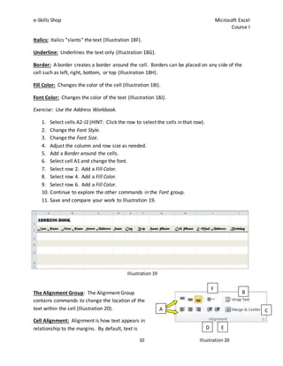
  • 10. e-Skills Shop Microsoft Excel Course I 10 Illustration 19 Italics: Italics slants the text (Illustration 18F). Underline: Underlines the text only (Illustration 18G). Border: A border creates a border around the cell. Borders can be placed on any side of the cell such as left, right, bottom, or top (Illustration 18H). Fill Color: Changes the color of the cell (Illustration 18I). Font Color: Changes the color of the text (Illustration 18J). Exercise: Use the Address Workbook. 1. Select cells A2-J2 (HINT: Click the row to select the cells in that row). 2. Change the Font Style. 3. Change the Font Size. 4. Adjust the column and row size as needed. 5. Add a Border around the cells. 6. Select cell A1 and change the font. 7. Select row 2. Add a Fill Color. 8. Select row 4. Add a Fill Color. 9. Select row 6. Add a Fill Color. 10. Continue to explore the other commands in the Font group. 11. Save and compare your work to Illustration 19. The Alignment Group: The Alignment Group contains commands to change the location of the text within the cell (Illustration 20). Cell Alignment: Alignment is how text appears in relationship to the margins. By default, text is A B C D E F Illustration 20
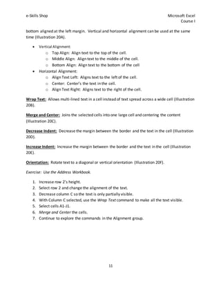
  • 11. e-Skills Shop Microsoft Excel Course I 11 bottom aligned at the left margin. Vertical and horizontal alignment can be used at the same time (Illustration 20A). Vertical Alignment: o Top Align: Align text to the top of the cell. o Middle Align: Align text to the middle of the cell. o Bottom Align: Align text to the bottom of the cell Horizontal Alignment: o Align Text Left: Aligns text to the left of the cell. o Center: Centers the text in the cell. o Align Text Right: Aligns text to the right of the cell. Wrap Text: Allows multi-lined text in a cell instead of text spread across a wide cell (Illustration 20B). Merge and Center: Joins the selected cells into one large cell and centering the content (Illustration 20C). Decrease Indent: Decrease the margin between the border and the text in the cell (Illustration 20D). Increase Indent: Increase the margin between the border and the text in the cell (Illustration 20E). Orientation: Rotate text to a diagonal or vertical orientation (Illustration 20F). Exercise: Use the Address Workbook. 1. Increase row 2s height. 2. Select row 2 and change the alignment of the text. 3. Decrease column C so the text is only partially visible. 4. With Column C selected, use the Wrap Text command to make all the text visible. 5. Select cells A1-J1. 6. Merge and Center the cells. 7. Continue to explore the commands in the Alignment group.
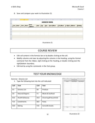
  • 12. e-Skills Shop Microsoft Excel Course I 12 Illustration 22 8. Save and compare your work to illustration 21. COURSE REVIEW Edit cell content in the formula bar or by double clicking on the cell. Modify columns and rows by adjusting the columns in the heading, using the Format command from the ribbon, right clicking on the heading, or double clicking over the right/bottom boundary. Edit text by using the commands in the Font group. TEST YOUR KNOWLEDGE Exercise: Grocery List 1. Type the following text into the cell indicated: Cell Text Cell Text A1 Grocery List B3 Produce D3 Natural/Organic F3 Meats & Seafood B13 Health& Beauty D13 Cleaning&Household F13 Condiments B23 Pasta D23 Baking F23 Cereal & Snacks Illustration 21
  • 13. e-Skills Shop Microsoft Excel Course I 13 B33 Dairy D33 Frozen F33 Other 2. Select cell A1. Increase the font size and change the font style. 3. Select cells A1-F2. Merge and Center. 4. Change the font size and style of remaining text. 5. Resize columns and rows referring to Illustration 22 as a guide. 6. Wrap text if needed. 7. Change the alignment. 8. Use the Fill Color command. 9. Add borders. 10. Save and compare your work to Illustration 22. Exercise: Gift Shopping List 1. Type the following text into the cell indicated: Cell Text Cell Text A1 Gift Shopping List F1 2012 B3 Christmas F3 Birthday B4 Gift Ideas C4 Store Name or URL D4 List Price E4 Purchase Price F4 Gift Ideas G4 Store Name or URL H4 List Price I4 Purchase Price A5 Spouse A6 Mom A7 Dad A8 Brother A9 Sister A10 Friend 2. Select cell A1. Increase the font size and change the font style. 3. Select cells B3-E3. Merge and Center.
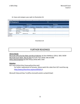
  • 14. e-Skills Shop Microsoft Excel Course I 14 4. Select cells F3-I3. Merge and Center. 5. Change the font size and style of remaining text. 6. Resize columns and rows. 7. Wrap text if needed. 8. Change the alignment. 9. Use the Fill Color command. 10. Add borders. 11. Type the following text into the cell indicated: Cell Text B5 I-Pod Touch C5 Apple D5 $200 B6 Crochet Blanket C6 JoAnn Fabrics D6 $30 B7 Gift Card C7 Tractor Supply D7 $40.00 B8 Harry Potter Box Set C8 Amazon.com D8 $43.76
  • 15. e-Skills Shop Microsoft Excel Course I 15 12. Save and compare your work to Illustration 23. FURTHER READINGS Library Books Microsoft Office for the Older and Wiser Publisher by Sean McManus (2011) 005.5 MCM Microsoft Excel 2010: Step by Step by Curtis Frye (2010) 005.54 C948 Office 2010 Simplified by Kate Shoup (2010) 005.5 SHO Websites GCF Learn Online (http://www.gcflearnfree.org/) For further explanations of formulas, please watch the video from GCF LearnFree.org (http://www.gcflearnfree.org/excel2010/6.2). Microsoft Help and How To (office.microsoft.com/en-us/word-help/) Illustration 23