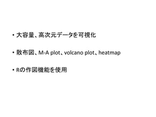
More Related Content
Similar to 2017年度 第5回バイオインフォマティクス実习 (13)
PPTX
ISMB2014読み会 Ragout—a reference-assisted assembly tool for bacterial genomesHaruka Ozaki?
More from Jun Nakabayashi (15)
2017年度 第5回バイオインフォマティクス実习
- 4. Rの設定
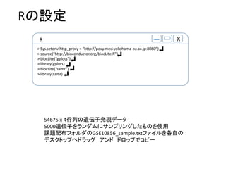
R X
> Sys.setenv(http_proxy = “http://poxy.med.yokohama-cu.ac.jp:8080”)
> source(“http://bioconductor.org/biocLite.R”)
> biocLite(“gplots”)
> library(gplots)
> biocLite(“samr”)
> library(samr)
54675 x 4行列の遺伝子発現データ
5000遺伝子をランダムにサンプリングしたものを使用
課題配布フォルダのGSE10856_sample.txtファイルを各自の
デスクトップへドラッグ アンド ドロップでコピー
- 5. scatter plot (散布図)
R X
> plot(x[,5], x[,6], pch = 20, col = “gray”, xlim = c(1,15), ylim = c(1,15), xlab = “IgG”,
+ ylab = “DcR3”, main = “scatter plot”)
散布図
データの分布を表示
Rでの行列の扱い
x[列,行]
plot(x軸, y軸, オプション)
pch:点のタイプ
col:色
xlim, ylim:x軸、y軸の範囲
xlab, ylab:x軸、y軸のラベル
main:タイトル
- 6. M-A plot
R X
> plot((x[,5] + x[,6])/2, x[,5] - x[,6]), pch = 20, col = “gray”, xlab = “A”,
+ ylab = “M”, main = “M-A plot”)
2群間比較
x軸:平均発現量
log2変換した値を使う
(log2(A)+log2(B)) / 2
y軸:発現比
log2(A/B)
- 7. volcano plot
2群間比較
x軸:発現比
y軸:p値
R X
> data.tmp <- list(x = x[,1:4], y = factor(c(“C”, “T”, “C”, “T”)), logged2 = TRUE)
> out <- samr(data.tmp, resp.type = “Two class unpaired”, nperms = 20)
> p.value <- samr.pvalues.from.perms(out$tt, out$ttstar)
> plot(x[,5] – x[,6], -log10(p.value), xlab = expression(paste(log[2], “(FC)”)),
+ ylab = expression(paste(log[10], “(p-value)”)), col = “gray”, main = “volcano plot”)
- 8. heatmap
R X
> heatmap.2(x[,1:4], col = greenred(75), cexRow = 0.1, cexCol = 0.8,
+ trace = “none”, density.info = “none”, main = “heatmap”)
散布図
データの分布を表示
Rでの行列の扱い
x[列,行]
gplots libraryのheatmap.2関数を
使用
cexRow, cexCol:x軸、y軸のラベル
文字の大きさ
col:greenred(階調)

![scatter plot (散布図)
R X
> plot(x[,5], x[,6], pch = 20, col = “gray”, xlim = c(1,15), ylim = c(1,15), xlab = “IgG”,
+ ylab = “DcR3”, main = “scatter plot”)
散布図
データの分布を表示
Rでの行列の扱い
x[列,行]
plot(x軸, y軸, オプション)
pch:点のタイプ
col:色
xlim, ylim:x軸、y軸の範囲
xlab, ylab:x軸、y軸のラベル
main:タイトル](https://image.slidesharecdn.com/2017bijishuno5-190806005710/85/2017-5-5-320.jpg)
![M-A plot
R X
> plot((x[,5] + x[,6])/2, x[,5] - x[,6]), pch = 20, col = “gray”, xlab = “A”,
+ ylab = “M”, main = “M-A plot”)
2群間比較
x軸:平均発現量
log2変換した値を使う
(log2(A)+log2(B)) / 2
y軸:発現比
log2(A/B)](https://image.slidesharecdn.com/2017bijishuno5-190806005710/85/2017-5-6-320.jpg)
![volcano plot
2群間比較
x軸:発現比
y軸:p値
R X
> data.tmp <- list(x = x[,1:4], y = factor(c(“C”, “T”, “C”, “T”)), logged2 = TRUE)
> out <- samr(data.tmp, resp.type = “Two class unpaired”, nperms = 20)
> p.value <- samr.pvalues.from.perms(out$tt, out$ttstar)
> plot(x[,5] – x[,6], -log10(p.value), xlab = expression(paste(log[2], “(FC)”)),
+ ylab = expression(paste(log[10], “(p-value)”)), col = “gray”, main = “volcano plot”)](https://image.slidesharecdn.com/2017bijishuno5-190806005710/85/2017-5-7-320.jpg)
![heatmap
R X
> heatmap.2(x[,1:4], col = greenred(75), cexRow = 0.1, cexCol = 0.8,
+ trace = “none”, density.info = “none”, main = “heatmap”)
散布図
データの分布を表示
Rでの行列の扱い
x[列,行]
gplots libraryのheatmap.2関数を
使用
cexRow, cexCol:x軸、y軸のラベル
文字の大きさ
col:greenred(階調)](https://image.slidesharecdn.com/2017bijishuno5-190806005710/85/2017-5-8-320.jpg)