
7.4
- 1. 7.4 ESTIMATING ’üŁ1 ŌĆō ’üŁ2 AND P1 ŌĆō P2
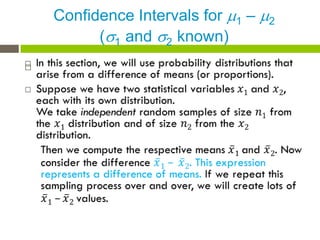
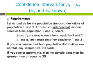
- 2. Independent Samples and Dependent Samples ’é© In this section, we will use samples from two populations to create confidence intervals for the difference between population parameters. ’éż we need to have a sample from each population ’éż Samples may be independent or dependent according to how they are selected
- 3. Independent Samples and Dependent Samples ’é© Two samples are independent is sample data drawn from one population are completely unrelated to the selection of sample data from the other population. ’éż Examples ’ü« Sample 1: test scores for 35 statistics students Sample 2: test scores for 42 biology students ’ü« Sample 1: heights of 27 adult females Sample 2: heights of 27 adult males ’ü« Sample 1: the SAT scores for 35 high school students who did not take an SAT preparation course Sample 2: the SAT scores for 40 high school students who did take an SAT preparation course
- 4. Independent Samples and Dependent Samples ’é© Two samples are dependent if each data value in one sample can be paired with a corresponding data value in the other sample. ’éż Examples ’ü« Sample 1: resting heart rates of 35 individuals before drinking coffee Sample 2: resting heart rates of the same individuals after drinking two cups of coffee ’ü« Sample 1: midterm exam scores of 14 chemistry students Sample 2: final exam scores of the same 14 chemistry students ’ü« Sample 1: the fuel mileage of 10 cars Sample 2: the fuel mileage of the same 10 cars using a fuel additive
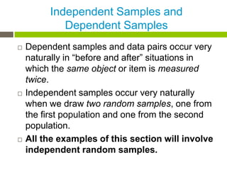
- 5. Independent Samples and Dependent Samples ’é© Dependent samples and data pairs occur very naturally in ŌĆ£before and afterŌĆØ situations in which the same object or item is measured twice. ’é© Independent samples occur very naturally when we draw two random samples, one from the first population and one from the second population. ’é© All the examples of this section will involve independent random samples.
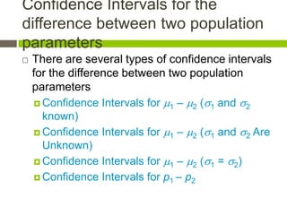
- 6. Confidence Intervals for the difference between two population parameters ’é© There are several types of confidence intervals for the difference between two population parameters ’éż Confidence Intervals for ’üŁ1 ŌĆō ’üŁ2 (’ü│1 and ’ü│2 known) ’éż Confidence Intervals for ’üŁ1 ŌĆō ’üŁ2 (’ü│1 and ’ü│2 Are Unknown) ’éż Confidence Intervals for ’üŁ1 ŌĆō ’üŁ2 (’ü│1 = ’ü│2) ’éż Confidence Intervals for p1 ŌĆō p2
- 7. Confidence Intervals for ’üŁ1 ŌĆō ’üŁ2 (’ü│1 and ’ü│2 known) ’é©
- 8. How to Interpret Confidence Intervals for Differences ’é©
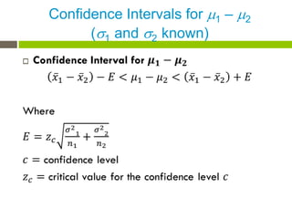
- 9. Confidence Intervals for ’üŁ1 ŌĆō ’üŁ2 (’ü│1 and ’ü│2 known) ’é©
- 10. Confidence Intervals for ’üŁ1 ŌĆō ’üŁ2 (’ü│1 and ’ü│2 known) ’é©
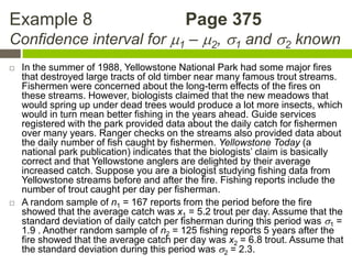
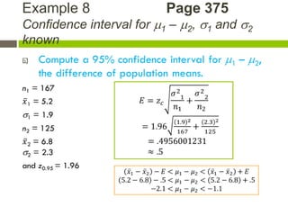
- 11. Example 8 Page 375 Confidence interval for ’üŁ1 ŌĆō ’üŁ2, ’ü│1 and ’ü│2 known ’é© In the summer of 1988, Yellowstone National Park had some major fires that destroyed large tracts of old timber near many famous trout streams. Fishermen were concerned about the long-term effects of the fires on these streams. However, biologists claimed that the new meadows that would spring up under dead trees would produce a lot more insects, which would in turn mean better fishing in the years ahead. Guide services registered with the park provided data about the daily catch for fishermen over many years. Ranger checks on the streams also provided data about the daily number of fish caught by fishermen. Yellowstone Today (a national park publication) indicates that the biologistsŌĆÖ claim is basically correct and that Yellowstone anglers are delighted by their average increased catch. Suppose you are a biologist studying fishing data from Yellowstone streams before and after the fire. Fishing reports include the number of trout caught per day per fisherman. ’é© A random sample of n1 = 167 reports from the period before the fire showed that the average catch was x1 = 5.2 trout per day. Assume that the standard deviation of daily catch per fisherman during this period was ’ü│1 = 1.9 . Another random sample of n2 = 125 fishing reports 5 years after the fire showed that the average catch per day was x2 = 6.8 trout. Assume that the standard deviation during this period was ’ü│2 = 2.3.
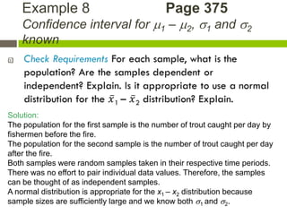
- 12. Example 8 Page 375 Confidence interval for ’üŁ1 ŌĆō ’üŁ2, ’ü│1 and ’ü│2 known ’é© Solution: The population for the first sample is the number of trout caught per day by fishermen before the fire. The population for the second sample is the number of trout caught per day after the fire. Both samples were random samples taken in their respective time periods. There was no effort to pair individual data values. Therefore, the samples can be thought of as independent samples. A normal distribution is appropriate for the x1 ŌĆō x2 distribution because sample sizes are sufficiently large and we know both ’ü│1 and ’ü│2.
- 13. Example 8 Page 375 Confidence interval for ’üŁ1 ŌĆō ’üŁ2, ’ü│1 and ’ü│2 known ’é©
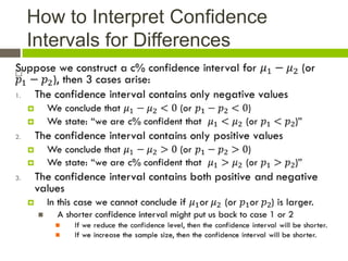
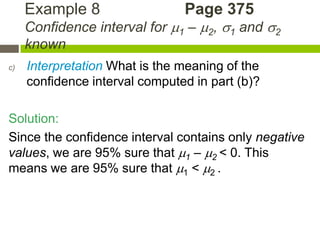
- 14. Example 8 Page 375 Confidence interval for ’üŁ1 ŌĆō ’üŁ2, ’ü│1 and ’ü│2 known c) Interpretation What is the meaning of the confidence interval computed in part (b)? Solution: Since the confidence interval contains only negative values, we are 95% sure that ’üŁ1 ŌĆō ’üŁ2 < 0. This means we are 95% sure that ’üŁ1 < ’üŁ2 .
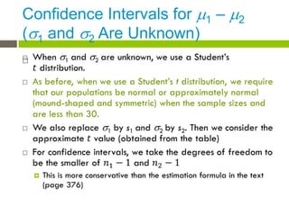
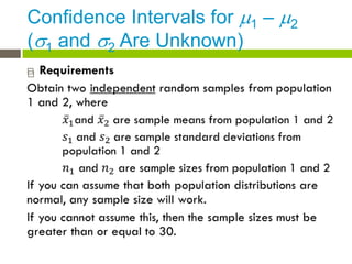
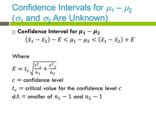
- 15. Confidence Intervals for ’üŁ1 ŌĆō ’üŁ2 (’ü│1 and ’ü│2 Are Unknown) ’é©
- 16. Confidence Intervals for ’üŁ1 ŌĆō ’üŁ2 (’ü│1 and ’ü│2 Are Unknown) ’é©
- 17. Confidence Intervals for ’üŁ1 ŌĆō ’üŁ2 (’ü│1 and ’ü│2 Are Unknown) ’é©
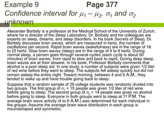
- 18. Example 9 Page 377 Confidence interval for ’üŁ1 ŌĆō ’üŁ2, ’ü│1 and ’ü│2 unknown Alexander Borbely is a professor at the Medical School of the University of Zurich, where he is director of the Sleep Laboratory. Dr. Borbely and his colleagues are experts on sleep, dreams, and sleep disorders. In his book Secrets of Sleep, Dr. Borbely discusses brain waves, which are measured in hertz, the number of oscillations per second. Rapid brain waves (wakefulness) are in the range of 16 to 25 hertz. Slow brain waves (sleep) are in the range of 4 to 8 hertz. During normal sleep, a person goes through several cycles (each cycle is about 90 minutes) of brain waves, from rapid to slow and back to rapid. During deep sleep, brain waves are at their slowest. In his book, Professor Borbely comments that alcohol is a poor sleep aid. In one study, a number of subjects were given 1/2 liter of red wine before they went to sleep. The subjects fell asleep quickly but did not remain asleep the entire night. Toward morning, between 4 and 6 A.M., they tended to wake up and have trouble going back to sleep. Suppose that a random sample of 29 college students was randomly divided into two groups. The first group of n1 = 15 people was given 1/2 liter of red wine before going to sleep. The second group of n2 = 14 people was given no alcohol before going to sleep. Everyone in both groups went to sleep at 11 P.M. The average brain wave activity (4 to 6 A.M.) was determined for each individual in the groups. Assume the average brain wave distribution in each group is moundshaped and symmetric.
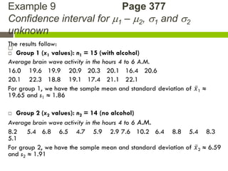
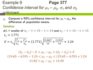
- 19. Example 9 Page 377 Confidence interval for ’üŁ1 ŌĆō ’üŁ2, ’ü│1 and ’ü│2 unknown ’é©
- 20. Example 9 Page 377 Confidence interval for ’üŁ1 ŌĆō ’üŁ2, ’ü│1 and ’ü│2 unknown ’é©
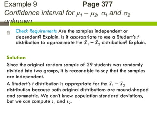
- 21. Example 9 Page 377 Confidence interval for ’üŁ1 ŌĆō ’üŁ2, ’ü│1 and ’ü│2 unknown ’é©
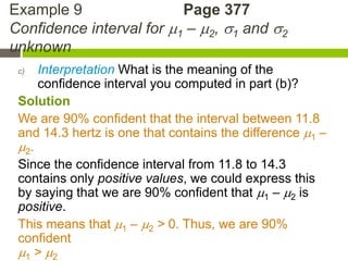
- 22. Example 9 Page 377 Confidence interval for ’üŁ1 ŌĆō ’üŁ2, ’ü│1 and ’ü│2 unknown c) Interpretation What is the meaning of the confidence interval you computed in part (b)? Solution We are 90% confident that the interval between 11.8 and 14.3 hertz is one that contains the difference ’üŁ1 ŌĆō ’üŁ2. Since the confidence interval from 11.8 to 14.3 contains only positive values, we could express this by saying that we are 90% confident that ’üŁ1 ŌĆō ’üŁ2 is positive. This means that ’üŁ1 ŌĆō ’üŁ2 > 0. Thus, we are 90% confident ’üŁ1 > ’üŁ2
- 23. Assignment ’é© Page 384 ’é© #1, 2, 4 ŌĆō 6, 7, 11, 23, 31