7.6 Solving Systems with Gaussian Elimination
- 1. 7.6 Gaussian Elimination Chapter 7 Systems of Equations and Inequalities
- 2. Concepts and Objectives ? The objectives for this section are ? Write the augmented matrix of a system of equations. ? Write the system of equations from an augmented matrix. ? Perform row operations on a matrix. ? Solve a system of linear equations using matrices.
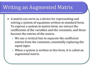
- 3. Writing an Augmented Matrix ? A matrix can serve as a device for representing and solving a system of equations written in standard form. To express a system in matrix form, we extract the coefficients of the variables and the constants, and these become the entries of the matrix. ? We use a vertical line to separate the coefficient entries from the constants, essentially replacing the equal signs. ? When a system is written in this form, it is called an augmented matrix.
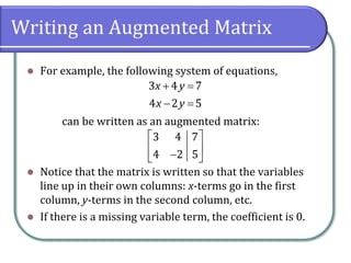
- 4. Writing an Augmented Matrix ? For example, the following system of equations, can be written as an augmented matrix: ? Notice that the matrix is written so that the variables line up in their own columns: x-terms go in the first column, y-terms in the second column, etc. ? If there is a missing variable term, the coefficient is 0. 3 4 7 4 2 5 x y x y + = ? = 3 4 7 4 2 5 ? ? ? ? ? ? ?
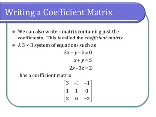
- 5. Writing a Coefficient Matrix ? We can also write a matrix containing just the coefficients. This is called the coefficient matrix. ? A 3 ¡Á 3 system of equations such as has a coefficient matrix 3 0 5 2 3 2 x y z x y x z ? ? = + = ? = 3 1 1 1 1 0 2 0 3 ? ? ? ? ? ? ? ? ? ? ? ? ?
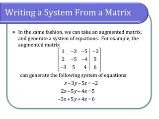
- 6. Writing a System From a Matrix ? In the same fashion, we can take an augmented matrix, and generate a system of equations. For example, the augmented matrix can generate the following system of equations: 1 3 5 2 2 5 4 5 3 5 4 6 ? ? ? ? ? ? ? ? ? ? ? ? ? ? ? ? 3 5 2 2 5 4 5 3 5 4 6 x y z x y z x y z ? ? = ? ? ? = ? + + =
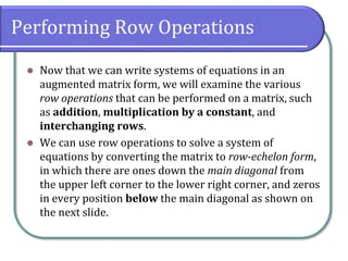
- 7. Performing Row Operations ? Now that we can write systems of equations in an augmented matrix form, we will examine the various row operations that can be performed on a matrix, such as addition, multiplication by a constant, and interchanging rows. ? We can use row operations to solve a system of equations by converting the matrix to row-echelon form, in which there are ones down the main diagonal from the upper left corner to the lower right corner, and zeros in every position below the main diagonal as shown on the next slide.
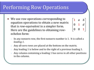
- 8. Performing Row Operations ? We use row operations corresponding to equation operations to obtain a new matrix that is row-equivalent in a simpler form. Here are the guidelines to obtaining row- echelon form: 1 1 0 0 0 1 a b d ? ? ? ? ? ? ? ? ? ? 1. In any nonzero row, the first nonzero number is 1. It is called a leading 1. 2. Any all-zero rows are placed at the bottom on the matrix. 3. Any leading 1 is below and to the right of a previous leading 1. 4. Any column containing a leading 1 has zeros in all other positions in the column.
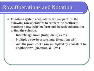
- 9. Row Operations and Notation ? To solve a system of equations we can perform the following row operations to convert the coefficient matrix to a row-echelon form and do back-substitution to find the solution. 1. Interchange rows. (Notation: ) 2. Multiply a row by a constant. (Notation: ) 3. Add the product of a row multiplied by a constant to another row. (Notation: ) i j R R ? i cR i j R cR +
- 10. Gaussian Elimination ? The primary tool we will be using is called Gaussian elimination, named after the prolific German mathematician Karl Friedrich Gauss. While there is no definitive order in which operations are to be performed, there are specific guidelines as to what type of moves can be made. ? To obtain a matrix in row-echelon form for finding solutions, we use row operations to obtain a 1 as the first entry so that row 1 can be used to convert the remaining rows.
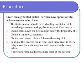
- 11. Procedure Given an augmented matrix, perform row operations to achieve row-echelon form. 1. The first equation should have a leading coefficient of 1. Interchange rows or multiply by a constant, if necessary. 2. Obtain zeros down the first column below the first entry of 1. 3. Obtain a 1 in row 2, column 2 4. Obtain zeros down column 2, below the entry of 1. 5. Continue this process for all rows until there is a 1 in every entry down the main diagonal and there are only zeros below. 6. If any rows contain all zeros, place them at the bottom.
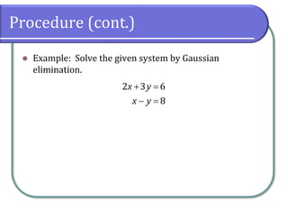
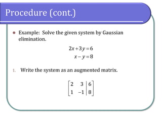
- 12. Procedure (cont.) ? Example: Solve the given system by Gaussian elimination. 2 3 6 8 x y x y + = ? =
- 13. Procedure (cont.) ? Example: Solve the given system by Gaussian elimination. 1. Write the system as an augmented matrix. 2 3 6 8 x y x y + = ? = 2 3 6 1 1 8 ? ? ? ? ? ? ?
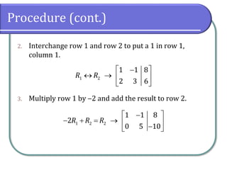
- 14. Procedure (cont.) 2. Interchange row 1 and row 2 to put a 1 in row 1, column 1. 3. Multiply row 1 by ?2 and add the result to row 2. 1 2 1 1 8 2 3 6 R R ? ? ? ? ¡ú ? ? ? ? 1 2 2 1 1 8 2 0 5 10 R R R ? ? ? ? + = ¡ú ? ? ? ? ?
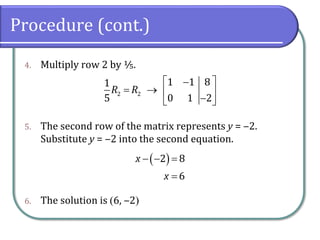
- 15. Procedure (cont.) 4. Multiply row 2 by ?. 5. The second row of the matrix represents y = ?2. Substitute y = ?2 into the second equation. 6. The solution is (6, ?2) 2 2 1 1 8 1 5 0 1 2 R R ? ? ? = ¡ú ? ? ? ? ? ( ) 2 8 6 x x ? ? = =
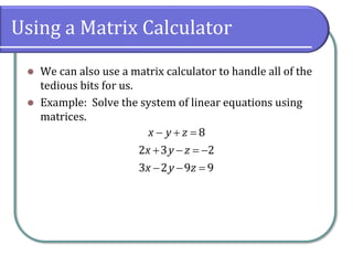
- 16. Using a Matrix Calculator ? We can also use a matrix calculator to handle all of the tedious bits for us. ? Example: Solve the system of linear equations using matrices. 8 2 3 2 3 2 9 9 x y z x y z x y z ? + = + ? = ? ? ? =
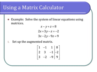
- 17. Using a Matrix Calculator ? Example: Solve the system of linear equations using matrices. 1. Set up the augmented matrix. 8 2 3 2 3 2 9 9 x y z x y z x y z ? + = + ? = ? ? ? = 1 1 1 8 2 3 1 2 3 2 9 9 ? ? ? ? ? ? ? ? ? ? ? ? ? ? ?
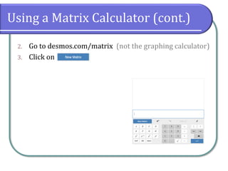
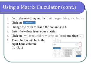
- 18. Using a Matrix Calculator (cont.) 2. Go to desmos.com/matrix (not the graphing calculator) 3. Click on
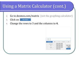
- 19. Using a Matrix Calculator (cont.) 2. Go to desmos.com/matrix (not the graphing calculator) 3. Click on 4. Change the rows to 3 and the columns to 4.
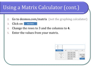
- 20. Using a Matrix Calculator (cont.) 2. Go to desmos.com/matrix (not the graphing calculator) 3. Click on 4. Change the rows to 3 and the columns to 4. 5. Enter the values from your matrix.
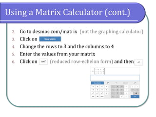
- 21. Using a Matrix Calculator (cont.) 2. Go to desmos.com/matrix (not the graphing calculator) 3. Click on 4. Change the rows to 3 and the columns to 4 5. Enter the values from your matrix 6. Click on (reduced row-echelon form) and then
- 22. Using a Matrix Calculator (cont.) 2. Go to desmos.com/matrix (not the graphing calculator) 3. Click on 4. Change the rows to 3 and the columns to 4 5. Enter the values from your matrix 6. Click on (reduced row-echelon form) and then 7. The solution will be in the right-hand column: (4, ?3, 1)
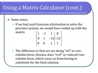
- 23. Using a Matrix Calculator (cont.) ? Some notes: ? If we had used Gaussian elimination to solve the previous system, we would have ended up with the matrix ? The difference is that we are doing ¡°ref¡± or row- echelon form; Desmos does ¡°rref¡± or reduced row- echelon form, which saves us from having to substitute for the final solution. 1 1 1 8 0 1 12 15 0 0 1 1 ? ? ? ? ? ? ? ? ? ? ? ? ?
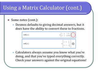
- 24. Using a Matrix Calculator (cont.) ? Some notes (cont.): ? Desmos defaults to giving decimal answers, but it does have the ability to convert these to fractions. ? Calculators always assume you know what you¡¯re doing, and that you¡¯ve typed everything correctly. Check your answers against the original equations!
- 25. Classwork ? College Algebra 2e ? 7.6: 6-14 (even); 7.5: 18, 20, 30-40 (even); 7.3: 52-58 (even) ? Quiz 7.5

