
adv-2015-16-solution-09
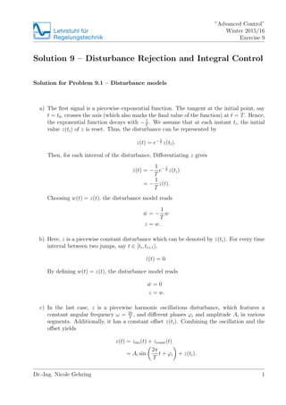
- 1. Lehrstuhlf¨ąr Regelungstechnik ˇ±Advanced Controlˇ± Winter 2015/16 Exercise 9 Solution 9 ¨C Disturbance Rejection and Integral Control Solution for Problem 9.1 ¨C Disturbance models a) The ?rst signal is a piecewise exponential function. The tangent at the initial point, say t = t0, crosses the axis (which also marks the ?nal value of the function) at t = T. Hence, the exponential function decays with ? 1 T . We assume that at each instant ti, the initial value z(ti) of z is reset. Thus, the disturbance can be represented by z(t) = e? t T z(ti). Then, for each interval of the disturbance, Di?erentiating z gives ¨Bz(t) = ? 1 T e? t T z(ti) = ? 1 T z(t). Choosing w(t) = z(t), the disturbance model reads ¨Bw = ? 1 T w z = w. b) Here, z is a piecewise constant disturbance which can be denoted by z(ti). For every time interval between two jumps, say t ˇĘ [ti, ti+1), ¨Bz(t) = 0. By de?ning w(t) = z(t), the disturbance model reads ¨Bw = 0 z = w. c) In the last case, z is a piecewise harmonic oscillations disturbance, which features a constant angular frequency ¦Ř = 2¦Đ T , and di?erent phases ?i and amplitude Ai in various segments. Additionally, it has a constant o?set z(ti). Combining the oscillation and the o?set yields z(t) = zsin(t) + zconst(t) = Ai sin 2¦Đ T t + ?i + z(ti). Dr.-Ing. Nicole Gehring 1
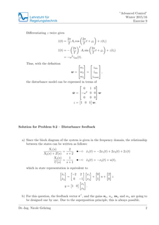
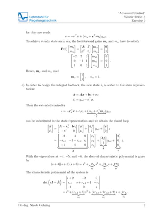
- 2. Lehrstuhlf¨ąr Regelungstechnik ˇ±Advanced Controlˇ± Winter 2015/16 Exercise 9 Di?erentiating z twice gives ¨Bz(t) = 2¦Đ T Ai cos 2¦Đ T t + ?i + z(ti) ˇ§z(t) = ? 2¦Đ T 2 Ai sin 2¦Đ T t + ?i + z(ti) = ?¦Ř2 zsin(t). Thus, with the de?nition w = ? ? ? w1 w2 w3 ? ? ? = ? ? ? zsin ¨Bzsin zconst ? ? ? , the disturbance model can be expressed in terms of ¨Bw = ? ? ? 0 1 0 ?¦Ř2 0 0 0 0 0 ? ? ? w z = 1 0 1 w. Solution for Problem 9.2 ¨C Disturbance feedback a) Since the block diagram of the system is given in the frequency domain, the relationship between the states can be written as follows: X1(s) X2(s) + Z(s) = 2 s + 2 t d ¨Bx1(t) = ?2x1(t) + 2x2(t) + 2z(t) X2(s) U(s) = 1 s + 1 t d ¨Bx2(t) = ?x2(t) + u(t), which in state representation is equivalent to ¨Bx1 ¨Bx2 = ?2 2 0 ?1 x1 x2 + 0 1 u + 2 0 z y = 1 0 x1 x2 . b) For this question, the feedback vector r , and the gains nx, nu, mx and mu are going to be designed one by one. Due to the superposition principle, this is always possible. Dr.-Ing. Nicole Gehring 2
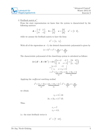
- 3. Lehrstuhlf¨ąr Regelungstechnik ˇ±Advanced Controlˇ± Winter 2015/16 Exercise 9 i) Feedback matrix r From the state representation we know that the system is characterized by the following matrices A = ?2 2 0 ?1 , b = 0 1 , e = 2 0 , c = 1 0 , while we assume the feedback matrix to have the form r = r1 r2 . With all of the eigenvalues at ?5, the desired characteristic polynomial is given by (s + 5)2 = s2 + 10 p1 s + 25 p0 . The characteristic polynomial of the closed-loop system is calculated as follows: det sI ? A + br = det s + 2 ?2 0 s + 1 + 0 0 r1 r2 = s + 2 ?2 r1 s + r2 + 1 = s2 + (r2 + 3) ¦Á1 s + 2r1 + 2r2 + 2 ¦Á0 Applying the coe?cient matching method s2 + (r2 + 3) ¦Á1 s + 2r1 + 2r2 + 2 ¦Á0 ! = s2 + 10 p1 s + 25 p0 , we obtain r2 + 3 ! = 10 2r1 + 2r2 + 2 ! = 25. Thus, r1 = 7 r2 = 4.5, i.e. the state feedback vector is r = 7 4.5 . Dr.-Ing. Nicole Gehring 3
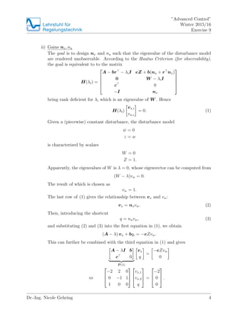
- 4. Lehrstuhlf¨ąr Regelungstechnik ˇ±Advanced Controlˇ± Winter 2015/16 Exercise 9 ii) Gains nx, nu The goal is to design nx and nu such that the eigenvalue of the disturbance model are rendered unobservable. According to the Hautus Criterion (for observability), the goal is equivalent to to the matrix H(¦Ëi) = ? ? ? ? ? A ? br ? ¦ËiI eZ + b(nu + r nx) 0 W ? ¦ËiI c 0 ?I nx ? ? ? ? ? being rank de?cient for ¦Ëi which is an eigenvalue of W . Hence H(¦Ëi) vx,i vw,i = 0. (1) Given a (piecewise) constant disturbance, the disturbance model ¨Bw = 0 z = w is characterized by scalars W = 0 Z = 1. Apparently, the eigenvalues of W is ¦Ë = 0, whose eigenvector can be computed from (W ? ¦Ë)vw = 0. The result of which is chosen as vw = 1. The last row of (1) gives the relationship between vx and vw: vx = nxvw. (2) Then, introducing the shortcut q = nuvw, (3) and substituting (2) and (3) into the ?rst equation in (1), we obtain (A ? ¦Ë) vx + bqi = ?eZvw. This can further be combined with the third equation in (1) and gives A ? ¦ËI b c 0 P (¦Ë) vx q = ?eZvw 0 ? ? ? ? ?2 2 0 0 ?1 1 1 0 0 ? ? ? ? ? ? vx,1 vx,2 q ? ? ? = ? ? ? ?2 0 0 ? ? ? . Dr.-Ing. Nicole Gehring 4
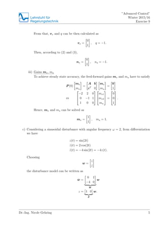
- 5. Lehrstuhlf¨ąr Regelungstechnik ˇ±Advanced Controlˇ± Winter 2015/16 Exercise 9 From that, vx and q can be then calculated as vx = 0 1 , q = ?1. Then, according to (2) and (3), nx = 0 1 , nu = ?1. iii) Gains mx, mu To achieve steady state accuracy, the feed-forward gains mx and mu have to satisfy P (0) mx mu = A b cT 0 mx mu = 0 1 ? ? ? ? ?2 2 0 0 ?1 1 1 0 0 ? ? ? ? ? ? mx1 mx2 mu ? ? ? = ? ? ? 0 0 1 ? ? ? . Hence, mx and mu can be solved as mx = 1 1 , mu = 1. c) Considering a sinusoidal disturbance with angular frequency ¦Ř = 2, from di?erentiation we have z(t) = sin(2t) ¨Bz(t) = 2 cos(2t) ˇ§z(t) = ?4 sin(2t) = ?4z(t). Choosing w = z ¨Bz the disturbance model can be written as ¨Bw = 0 1 ?4 0 W w z = 1 0 Z w. Dr.-Ing. Nicole Gehring 5
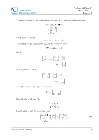
- 6. Lehrstuhlf¨ąr Regelungstechnik ˇ±Advanced Controlˇ± Winter 2015/16 Exercise 9 The eigenvalues of W are calculated as the roots ¦Ë of the characteristic equation 0 = det(¦ËI ? W ) = ¦Ë ?1 4 ¦Ë = ¦Ë2 + 4, which gives the result ¦Ë1 = 2j, ¦Ë2 = ?2j. The corresponding eigenvectors vw,i can be calculated from (W ? ¦ËiI)vw,i = 0. For ¦Ë1, ?2j 1 ?4 ?2j vw,1,1 vw,1,2 = 0 vw,1 = 1 2j is an eigenvector, for ¦Ë2, 2j 1 ?4 2j vw,2,1 vw,2,2 = 0 vw,2 = 1 ?2j . Thus the matrix of the eigenvectors reads V w = 1 1 2j ?2j . Equivalently to (2) and (3) V x = NxV w q = nu V w. Substituting ¦Ë1 and ¦Ë2 respectively into A ? ¦ËiI b c 0 P (¦Ëi) vx q = ?eZvw 0 , (4) Dr.-Ing. Nicole Gehring 6
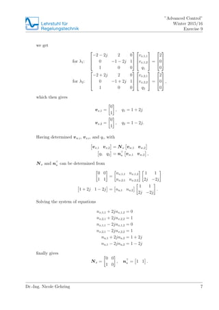
- 7. Lehrstuhlf¨ąr Regelungstechnik ˇ±Advanced Controlˇ± Winter 2015/16 Exercise 9 we get for ¦Ë1: ? ? ? ?2 ? 2j 2 0 0 ?1 ? 2j 1 1 0 0 ? ? ? ? ? ? vx,1,1 vx,1,2 q1 ? ? ? = ? ? ? 2 0 0 ? ? ? for ¦Ë2: ? ? ? ?2 + 2j 2 0 0 ?1 + 2j 1 1 0 0 ? ? ? ? ? ? vx,2,1 vx,2,2 q2 ? ? ? = ? ? ? 2 0 0 ? ? ? , which then gives vx,1 = 0 1 , q1 = 1 + 2j vx,2 = 0 1 , q2 = 1 ? 2j. Having determined vw,i, vx,i, and qi, with vx,1 vx,2 = Nx vw,1 vw,2 q1 q2 = nu vw,1 vw,2 , Nx and nu can be determined from 0 0 1 1 = nx,1,1 nx,1,2 nx,2,1 nx,2,2 1 1 2j ?2j 1 + 2j 1 ? 2j = nu,1 nu,2 1 1 2j ?2j . Solving the system of equations nx,1,1 + 2jnx,1,2 = 0 nx,2,1 + 2jnx,2,2 = 1 nx,1,1 ? 2jnx,1,2 = 0 nx,2,1 ? 2jnx,2,2 = 1 nu,1 + 2jnu,2 = 1 + 2j nu,1 ? 2jnu,2 = 1 ? 2j ?nally gives Nx = 0 0 1 0 , nu = 1 1 . Dr.-Ing. Nicole Gehring 7
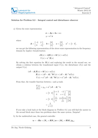
- 8. Lehrstuhlf¨ąr Regelungstechnik ˇ±Advanced Controlˇ± Winter 2015/16 Exercise 9 Solution for Problem 9.3 ¨C Integral control and disturbance observer a) Given the state representation ¨Bx = Ax + bu + ez y = c x where A = ?2 2 0 ?1 , b = 0 1 , e = 2 0 , c = 1 0 , we can get the following representation of the above state representation in the frequency domain by Laplace transformation: sX(s) = AX(s) + bU(s) + eZ(s) Y (s) = c X(s) By solving the ?rst equation for X(s) and replacing the result in the second one, we obtain a relation between the transformed input U(s), the disturbance Z(s) and the output Y (s): (sI ? A)X(s) = bU(s) + eZ(s) X(s) = (sI ? A)?1 bU(s) + (sI ? A)?1 eZ(s) Y (s) = c (sI ? A)?1 bU(s) + c (sI ? A)?1 eZ(s). From that, the transfer function between z and y reads Y (s) Z(s) = gzy = c (sI ? A)?1 e = 1 0 s + 2 ?2 0 s + 1 ?1 2 0 = 1 0 1 s+2 2 (s+1)(s+2) 0 1 s+1 2 0 = 2 s + 2 . If you take a look back at the block diagram in Problem 9.2, you will ?nd the answer in the second block since these two problems share the same system. Surprise! b) In the undisturbed case, the general controller u = ?Rx + (Nu + RNx)w + (Mu + RMx)yref Dr.-Ing. Nicole Gehring 8
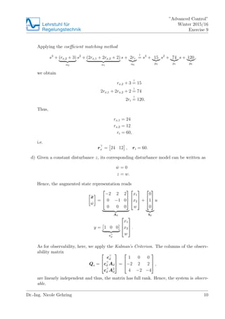
- 9. Lehrstuhlf¨ąr Regelungstechnik ˇ±Advanced Controlˇ± Winter 2015/16 Exercise 9 for this case reads u = ?r x + (mu + r mx)yref. To achieve steady state accuracy, the feed-forward gains mx and mu have to satisfy P (0) mx mu = A b cT 0 mx mu = 0 1 ? ? ? ?2 2 0 0 ?1 1 1 0 0 ? ? ? ? ? ? mx1 mx2 mu ? ? ? = ? ? ? 0 0 1 ? ? ? . Hence, mx and mu read mx = 1 1 , mu = 1. c) In order to design the integral feedback, the new state xi is added to the state represen- tation: ¨Bx = Ax + bu + ez ¨Bxi = yref ? c x. Then the extended controller u = ?rx x + rixi + (mu + rx mx) f yref can be substituted in the state representation and we obtain the closed loop ¨Bx ¨Bxi = A ? rx bri ?c 0 x xi + bf 1 yref + e 0 z = ? ? ? ?2 2 0 ?rx,1 ?1 ? rx,2 ri ?1 0 0 ? ? ? ?A ? ? ? x1 x2 xi ? ? ? + bf 1 ?b yref + ? ? ? 2 0 0 ? ? ? ?e z. With the eigenvalues at ?4, ?5, and ?6, the desired characteristic polynomial is given by (s + 4)(s + 5)(s + 6) = s3 + 15 p2 s2 + 74 p1 s + 120 p0 . The characteristic polynomial of the system is det sI ? ?A = s + 2 ?2 0 rx,1 s + rx,2 + 1 ?ri 1 0 s = s3 + (rx,2 + 3) ¦Á2 s2 + (2rx,1 + 2rx,2 + 2) ¦Á1 s + 2r1 ¦Á0 . Dr.-Ing. Nicole Gehring 9
- 10. Lehrstuhlf¨ąr Regelungstechnik ˇ±Advanced Controlˇ± Winter 2015/16 Exercise 9 Applying the coe?cient matching method s3 + (rx,2 + 3) ¦Á2 s2 + (2rx,1 + 2rx,2 + 2) ¦Á1 s + 2ri ¦Á0 ! = s3 + 15 p2 s2 + 74 p1 s + 120 p0 , we obtain rx,2 + 3 ! = 15 2rx,1 + 2rx,2 + 2 ! = 74 2ri ! = 120. Thus, rx,1 = 24 rx,2 = 12 ri = 60, i.e. rx = 24 12 , ri = 60. d) Given a constant disturbance z, its corresponding disturbance model can be written as ¨Bw = 0 z = w. Hence, the augmented state representation reads ¨Bx ¨Bw = ? ? ? ?2 2 2 0 ?1 0 0 0 0 ? ? ? Ad ? ? ? x1 x2 w ? ? ? + ? ? ? 0 1 0 ? ? ? bd u y = 1 0 0 cd ? ? ? x1 x2 w ? ? ? . As for observability, here, we apply the KalmanˇŻs Criterion. The columns of the observ- ability matrix Qo = ? ? ? cd cd Ad cd A2 d ? ? ? = ? ? ? 1 0 0 ?2 2 2 4 ?2 ?4 ? ? ? , are linearly independent and thus, the matrix has full rank. Hence, the system is observ- able. Dr.-Ing. Nicole Gehring 10
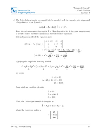
- 11. Lehrstuhlf¨ąr Regelungstechnik ˇ±Advanced Controlˇ± Winter 2015/16 Exercise 9 e) The desired characteristic polynomial is to be matched with the characteristic polynomial of the observer error dynamics: det sI ? Ad + lcd ! = (s + 10)3 . Here, the unknown correction matrix L = l has dimension 3 ˇÁ 1 since one measurement is used to correct the three-dimensional state of observer dynamics. Calculating each side of the equation gives det sI ? Ad + lcd = s + l1 + 2 ?2 ?2 l2 s + 1 0 l3 0 s = s3 + (l1 + 3) ¦Á2 s2 + (l1 + 2l2 + 2l3 + 2) ¦Á1 s + 2l3 ¦Á0 , (s + 10)3 = s3 + 30 p2 s2 + 300 p1 s + 1000 p0 . Applying the coe?cient matching method s3 + (l1 + 3) ¦Á2 s2 + (l1 + 2l2 + 2l3 + 2) ¦Á1 s + 2l3 ¦Á0 ! = s3 + 30 p2 s2 + 300 p1 s + 1000 p0 , we obtain l1 + 3 = 30 l1 + 2l2 + 2l3 + 2 = 300 2l3 = 1000, from which we can then calculate l1 = 27 l2 = ?364.5 l3 = 500. Thus, the Luenberger observer is designed as ¨B?x = Ad ?x + bdu + l(y ? ?y), where the correction matrix is l = ? ? ? 27 ?364.5 500 ? ? ? . Dr.-Ing. Nicole Gehring 11
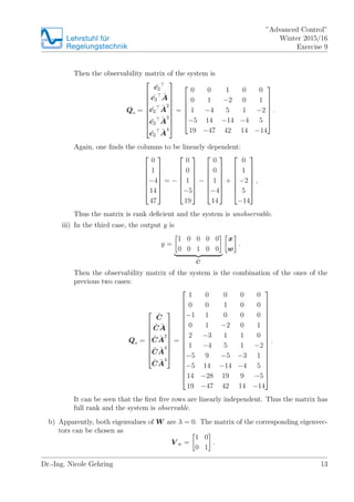
- 12. Lehrstuhlf¨ąr Regelungstechnik ˇ±Advanced Controlˇ± Winter 2015/16 Exercise 9 Solution for Problem 9.4 ¨C Three-tank system a) Inserting the known matrices into the state representation of the three-tank system gives ¨Bx ¨Bw = ? ? ? ? ? ? ? ?1 1 0 0 0 1 ?2 1 1 0 0 1 ?2 0 1 0 0 0 0 0 0 0 0 0 0 ? ? ? ? ? ? ? ?A x w + ? ? ? ? ? ? ? 1 0 0 0 0 1 0 0 0 0 ? ? ? ? ? ? ? ?B u. i) In the ?rst case, the output y is y = 1 0 0 0 0 ?c1 x w . Then the observability matrix of the (augmented) system is Qo = ? ? ? ? ? ? ? ? ? ?c1 ?c1 ?A ?c1 ?A 2 ?c1 ?A 3 ?c1 ?A 4 ? ? ? ? ? ? ? ? ? = ? ? ? ? ? ? ? 1 0 0 0 0 ?1 1 0 0 0 2 ?3 1 1 0 ?5 9 ?5 ?3 1 14 ?28 19 9 ?5 ? ? ? ? ? ? ? , where the last three columns are linearly dependent: ? ? ? ? ? ? ? 0 0 1 ?5 19 ? ? ? ? ? ? ? = ? ? ? ? ? ? ? 0 0 1 ?3 9 ? ? ? ? ? ? ? ? 2 ? ? ? ? ? ? ? 0 0 0 1 ?5 ? ? ? ? ? ? ? . Thus the matrix is rank de?cient and the system is unobservable. ii) In the second case, the output y is y = 0 0 1 0 0 ?c2 x w . Dr.-Ing. Nicole Gehring 12
- 13. Lehrstuhlf¨ąr Regelungstechnik ˇ±Advanced Controlˇ± Winter 2015/16 Exercise 9 Then the observability matrix of the system is Qo = ? ? ? ? ? ? ? ? ? ?c2 ?c2 ?A ?c2 ?A 2 ?c2 ?A 3 ?c2 ?A 4 ? ? ? ? ? ? ? ? ? = ? ? ? ? ? ? ? 0 0 1 0 0 0 1 ?2 0 1 1 ?4 5 1 ?2 ?5 14 ?14 ?4 5 19 ?47 42 14 ?14 ? ? ? ? ? ? ? . Again, one ?nds the columns to be linearly dependent: ? ? ? ? ? ? ? 0 1 ?4 14 47 ? ? ? ? ? ? ? = ? ? ? ? ? ? ? ? 0 0 1 ?5 19 ? ? ? ? ? ? ? ? ? ? ? ? ? ? ? 0 0 1 ?4 14 ? ? ? ? ? ? ? + ? ? ? ? ? ? ? 0 1 ?2 5 ?14 ? ? ? ? ? ? ? , Thus the matrix is rank de?cient and the system is unobservable. iii) In the third case, the output y is y = 1 0 0 0 0 0 0 1 0 0 ?C x w . Then the observability matrix of the system is the combination of the ones of the previous two cases: Qo = ? ? ? ? ? ? ? ? ? ?C ?C ?A ?C ?A 2 ?C ?A 3 ?C ?A 4 ? ? ? ? ? ? ? ? ? = ? ? ? ? ? ? ? ? ? ? ? ? ? ? ? ? ? ? ? 1 0 0 0 0 0 0 1 0 0 ?1 1 0 0 0 0 1 ?2 0 1 2 ?3 1 1 0 1 ?4 5 1 ?2 ?5 9 ?5 ?3 1 ?5 14 ?14 ?4 5 14 ?28 19 9 ?5 19 ?47 42 14 ?14 ? ? ? ? ? ? ? ? ? ? ? ? ? ? ? ? ? ? ? . It can be seen that the ?rst ?ve rows are linearly independent. Thus the matrix has full rank and the system is observable. b) Apparently, both eigenvalues of W are ¦Ë = 0. The matrix of the corresponding eigenvec- tors can be chosen as V w = 1 0 0 1 . Dr.-Ing. Nicole Gehring 13
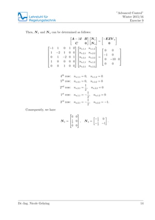
- 14. Lehrstuhlf¨ąr Regelungstechnik ˇ±Advanced Controlˇ± Winter 2015/16 Exercise 9 Then, Nx and Nu can be determined as follows: A ? ¦ËI B C 0 Nx Nu = ?EZV w 0 ? ? ? ? ? ? ? ?1 1 0 1 0 1 ?2 1 0 0 0 1 ?2 0 1 1 0 0 0 0 0 0 1 0 0 ? ? ? ? ? ? ? ? ? ? ? ? ? ? nx,1,1 nx,1,2 nx,2,1 nx,2,2 nx,3,1 nx,3,2 nu,1,1 nu,1,2 nu,2,1 nu,2,2 ? ? ? ? ? ? ? = ? ? ? ? ? 0 0 ?1 0 0 ?10 0 0 0 ? ? ? ? ? 4th row: nx,1,1 = 0, nx,1,2 = 0 5th row: nx,3,1 = 0, nx,3,2 = 0 2nd row: nx,2,1 = 1 2 , nx,2,2 = 0 1st row: nu,1,1 = ? 1 2 , nu,1,2 = 0 3rd row: nu,2,1 = ? 1 2 , nu,2,2 = ?1. Consequently, we have Nx = ? ? ? 0 0 1 2 0 0 0 ? ? ? , Nu = ?1 2 0 ?1 2 ?1 . Dr.-Ing. Nicole Gehring 14