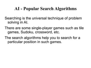


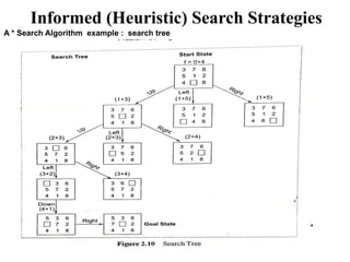
![Informed (Heuristic) Search Strategies
A * Search Algorithm
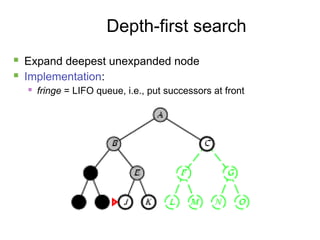
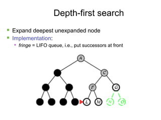
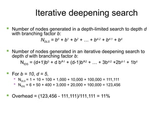
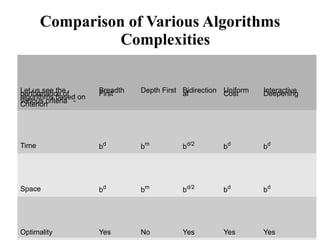
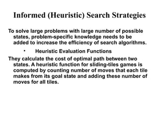
example: Let us consider eight puzzle problem and solve it by A*
algorithm.
Let define the evaluation function as:
f(X) = g(X) + h(X), where [ f(startstate)= 0 + 4 = 4 ]
h(X) = the number of tiles not in their goal position in a given state X
g(X) = depth of node X in the search tree
Start state Goal State
3 7 6
5 1 2
4 8
5 3 6
7 2
4 1 8](https://image.slidesharecdn.com/ai-search-metods-250106153229-6f3d9b59/85/AI-search-metodsandeverythingelsenot-ppt-43-320.jpg)
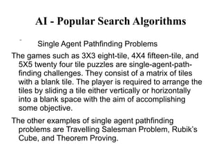
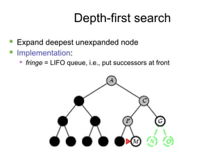
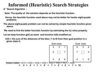
![Informed (Heuristic) Search Strategies
A * Search Algorithm
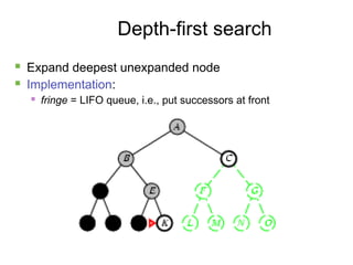
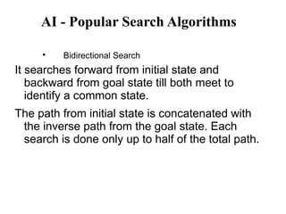
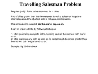
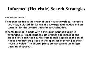
example: Let us consider eight puzzle problem and solve it by A*
algorithm.
Let define the evaluation function as:
f(X) = g(X) + h(X), where [ f(startstate)= 0 + 4 ]
h(X) = the number of tiles not in their goal position in a given state X = 4
g(X) = depth of node X in the search tree [for start node = 0]
Start state Goal State
3 7 6
5 1 2
4 8
5 3 6
7 2
4 1 8](https://image.slidesharecdn.com/ai-search-metods-250106153229-6f3d9b59/85/AI-search-metodsandeverythingelsenot-ppt-44-320.jpg)
AI-search-metodsandeverythingelsenot.ppt
- 1. AI - Popular Search Algorithms Searching is the universal technique of problem solving in AI. There are some single-player games such as tile games, Sudoku, crossword, etc. The search algorithms help you to search for a particular position in such games.
- 2. AI - Popular Search Algorithms ´Ç¡ Single Agent Pathfinding Problems The games such as 3X3 eight-tile, 4X4 fifteen-tile, and 5X5 twenty four tile puzzles are single-agent-path- finding challenges. They consist of a matrix of tiles with a blank tile. The player is required to arrange the tiles by sliding a tile either vertically or horizontally into a blank space with the aim of accomplishing some objective. The other examples of single agent pathfinding problems are Travelling Salesman Problem, RubikÔÇÖs Cube, and Theorem Proving.
- 3. AI - Popular Search Algorithms ´Ç¡ Search Terminology Problem Space ´╝ì It is the environment in which the search takes place. (A set of states and set of operators to change those states) Problem Instance ´╝ì It is Initial state + Goal state. Problem Space Graph ´╝ì It represents problem state. States are shown by nodes and operators are shown by edges. Depth of a problem ´╝ì Length of a shortest path or shortest sequence of operators from Initial State to goal state. Space Complexity ´╝ì The maximum number of nodes that are stored in memory. Time Complexity ´╝ì The maximum number of nodes that are created. Admissibility ´╝ì A property of an algorithm to always find an optimal solution. Branching Factor ´╝ì The average number of child nodes in the problem space graph. Depth ´╝ì Length of the shortest path from initial state to goal state.
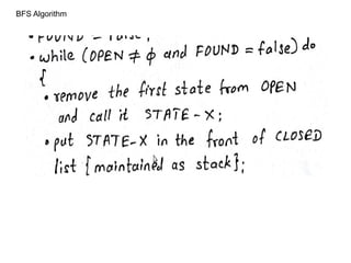
- 4. AI - Popular Search Algorithms ´ü¼ Breadth-First Search (Exhaustive Search) It starts from the root node, explores the neighboring nodes first and moves towards the next level neighbors. It generates one tree at a time until the solution is found. It can be implemented using FIFO queue data structure. This method provides shortest path to the solution. If branching factor (average number of child nodes for a given node) = b and depth = d, then number of nodes at level d = bd. The total no of nodes created in worst case is b + b2 + b3 + ÔǪ + bd. Disadvantage ´╝ì Since each level of nodes is saved for creating next one, it consumes a lot of memory space. Space requirement to store nodes is exponential. Its complexity depends on the number of nodes. It can check duplicate nodes.
- 5. AI - Popular Search Algorithms ´ü¼ Breadth-First Search
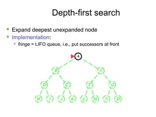
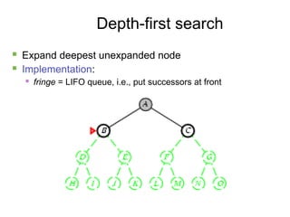
- 9. AI - Popular Search Algorithms Depth-First Search Exhaustive Search It is implemented in recursion with LIFO stack data structure. It creates the same set of nodes as Breadth-First method, only in the different order. As the nodes on the single path are stored in each iteration from root to leaf node, the space requirement to store nodes is linear. With branching factor b and depth as m, the storage space is bm. Disadvantage ´╝ì This algorithm may not terminate and go on infinitely on one path. The solution to this issue is to choose a cut-off depth. If the ideal cut-off is d, and if chosen cut-off is lesser than d, then this algorithm may fail. If chosen cut-off is more than d, then execution time increases. Its complexity depends on the number of paths. It cannot check duplicate nodes.
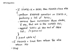
- 10. Algorithm (DFS) Input: START and GOAL states of the problem LOCAL Variables: OPEN, CLOSED, RECORD_X, SUCCESSORS, FOUND Output: A path sequence from START to GOAL state, if one exists otherwise return No Method: . initialize OPEN list with (START, nil) and set CLOSED = ╬ª; . FOUND = false; . while (OPEN Ôëá Ðä and FOUND = false) do { . remove the first record (initially (START, nil)) from OPEN list and call it RECORD-X; . put RECORD-X in the front of CLOSED list (maintained as stack); . if (START_X of RECORDD_X = GOAL) then FOUND = true else { . perform EXPAND operation on STATE-X producing a list of records called SUCCESSORS; create each record by associating parent link with its state; . remove from SUCCESSORS any record that is already in the CLOSED list; . insert SUCCESSORS in the front of the OPEN list /*stack*/ } } /* end while*/ . if found = true then return the path by tracing through the pointers to the parents on the CLOSED list else return NO . Stop
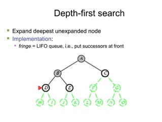
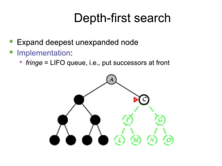
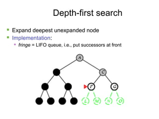
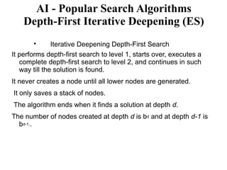
- 11. 11 Depth-first search ´ü« Expand deepest unexpanded node ´ü« Implementation: ´ü« fringe = LIFO queue, i.e., put successors at front
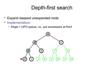
- 12. 12 Depth-first search ´ü« Expand deepest unexpanded node ´ü« Implementation: ´ü« fringe = LIFO queue, i.e., put successors at front
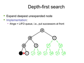
- 13. 13 Depth-first search ´ü« Expand deepest unexpanded node ´ü« Implementation: ´ü« fringe = LIFO queue, i.e., put successors at front
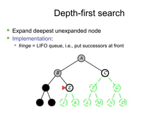
- 14. 14 Depth-first search ´ü« Expand deepest unexpanded node ´ü« Implementation: ´ü« fringe = LIFO queue, i.e., put successors at front
- 15. 15 Depth-first search ´ü« Expand deepest unexpanded node ´ü« Implementation: ´ü« fringe = LIFO queue, i.e., put successors at front
- 16. 16 Depth-first search ´ü« Expand deepest unexpanded node ´ü« Implementation: ´ü« fringe = LIFO queue, i.e., put successors at front
- 17. 17 Depth-first search ´ü« Expand deepest unexpanded node ´ü« Implementation: ´ü« fringe = LIFO queue, i.e., put successors at front
- 18. 18 Depth-first search ´ü« Expand deepest unexpanded node ´ü« Implementation: ´ü« fringe = LIFO queue, i.e., put successors at front
- 19. 19 Depth-first search ´ü« Expand deepest unexpanded node ´ü« Implementation: ´ü« fringe = LIFO queue, i.e., put successors at front
- 20. 20 Depth-first search ´ü« Expand deepest unexpanded node ´ü« Implementation: ´ü« fringe = LIFO queue, i.e., put successors at front
- 21. 21 Depth-first search ´ü« Expand deepest unexpanded node ´ü« Implementation: ´ü« fringe = LIFO queue, i.e., put successors at front
- 22. 22 Depth-first search ´ü« Expand deepest unexpanded node ´ü« Implementation: ´ü« fringe = LIFO queue, i.e., put successors at front
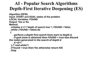
- 23. AI - Popular Search Algorithms Depth-First Iterative Deepening (ES) ´ü¼ Iterative Deepening Depth-First Search It performs depth-first search to level 1, starts over, executes a complete depth-first search to level 2, and continues in such way till the solution is found. It never creates a node until all lower nodes are generated. It only saves a stack of nodes. The algorithm ends when it finds a solution at depth d. The number of nodes created at depth d is bd and at depth d-1 is bd-1..
- 24. Algorithm (DFID) Input: START and GOAL states of the problem LOCAL Variables: FOUND Output: Yes or No Method: . initialize d =1 /*depth of search tree */, FOUND = false; . while ( FOUND = false) do { . perform a depth first search from start to depth d. . if goal state is obtained then FOUND = true else discard the nodes generated in the search of depth d . d =d+1 } /* end while*/ . if found = true then Yes otherwise return NO . Stop AI - Popular Search Algorithms Depth-First Iterative Deepening (ES)
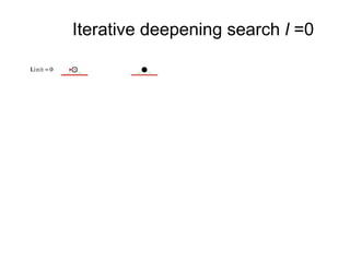
- 25. 26 Iterative deepening search l =0
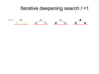
- 26. 27 Iterative deepening search l =1
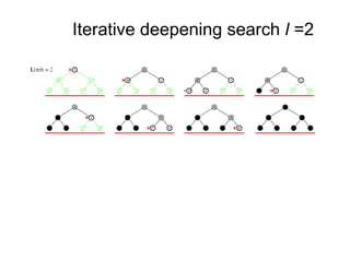
- 27. 28 Iterative deepening search l =2
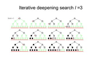
- 28. 29 Iterative deepening search l =3
- 29. 30 Iterative deepening search ´ü« Number of nodes generated in a depth-limited search to depth d with branching factor b: NDLS = b0 + b1 + b2 + ÔǪ + bd-2 + bd-1 + bd ´ü« Number of nodes generated in an iterative deepening search to depth d with branching factor b: NIDS = (d+1)b0 + d b^1 + (d-1)b^2 + ÔǪ + 3bd-2 +2bd-1 + 1bd ´ü« For b = 10, d = 5, ´ü« NDLS = 1 + 10 + 100 + 1,000 + 10,000 + 100,000 = 111,111 ´ü« NIDS = 6 + 50 + 400 + 3,000 + 20,000 + 100,000 = 123,456 ´ü« Overhead = (123,456 - 111,111)/111,111 = 11%
- 30. AI - Popular Search Algorithms ´ü¼ Bidirectional Search It searches forward from initial state and backward from goal state till both meet to identify a common state. The path from initial state is concatenated with the inverse path from the goal state. Each search is done only up to half of the total path.
- 31. https://efficientcodeblog.wordpress.com/2017/12/13/bidirectional-search-two-end-bfs/ Algorithm Bidirectional example AI - Popular Search Algorithms
- 32. AI - Popular Search Algorithms ´ü¼ Uniform Cost Search Sorting is done in increasing cost of the path to a node. It always expands the least cost node. It is identical to Breadth First search if each transition has the same cost. It explores paths in the increasing order of cost. Disadvantage ´╝ì There can be multiple long paths with the cost Ôëñ C*. Uniform Cost search must explore them all.
- 33. Comparison of Various Algorithms Complexities Let us see the performance of algorithms based on various criteria ´╝ì Criterion Breadth First Depth First Bidirection al Uniform Cost Interactive Deepening Time bd bm bd/2 bd bd Space bd bm bd/2 bd bd Optimality Yes No Yes Yes Yes
- 34. Informed (Heuristic) Search Strategies To solve large problems with large number of possible states, problem-specific knowledge needs to be added to increase the efficiency of search algorithms. ´ü¼ Heuristic Evaluation Functions They calculate the cost of optimal path between two states. A heuristic function for sliding-tiles games is computed by counting number of moves that each tile makes from its goal state and adding these number of moves for all tiles.
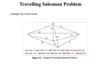
- 35. Travelling Salesman Problem ´ü¼ Travelling Salesman Problem In this algorithm, the objective is to find a low-cost tour that starts from a city, visits all cities en-route exactly once and ends at the same starting city. Start Find out all (n -1)! Possible solutions, where n is the total number of cities. Determine the minimum cost by finding out the cost of each of these (n -1)! solutions. Finally, keep the one with the minimum cost. End
- 36. Travelling Salesman Problem Requires (n-1)! Paths to be examined for n cities. If no of cities grows, then the time required to wait a salesman to get the information about the shortest path is not a practical situation. This phenomenon is called combinatorial explosion. It can be improved little by following technique: 1. Start generating complete paths, keeping track of the shortest path found so far. .2. Stop exploring any path as soon as its partial length becomes greater than the shortest path length found so far. Example: fig 2.9 from book
- 37. Travelling Salesman Problem Example: fig 2.9 from book
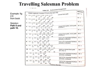
- 38. Travelling Salesman Problem Example: fig 2.9 from book Solution: Path 6 and path 10.
- 39. Informed (Heuristic) Search Strategies To solve large problems with large number of possible states, problem-specific knowledge needs to be added to increase the efficiency of search algorithms. ´ü¼ Heuristic Evaluation Functions They calculate the cost of optimal path between two states. A heuristic function for sliding-tiles games is computed by counting number of moves that each tile makes from its goal state and adding these number of moves for all tiles.
- 40. Informed (Heuristic) Search Strategies Pure Heuristic Search It expands nodes in the order of their heuristic values. It creates two lists, a closed list for the already expanded nodes and an open list for the created but unexpanded nodes. In each iteration, a node with a minimum heuristic value is expanded, all its child nodes are created and placed in the closed list. Then, the heuristic function is applied to the child nodes and they are placed in the open list according to their heuristic value. The shorter paths are saved and the longer ones are disposed.
- 41. Informed (Heuristic) Search Strategies A * Search It is best-known form of Best First search. It avoids expanding paths that are already expensive, but expands most promising paths first. f(n) = g(n) + h(n), where g(n) the cost (so far) to reach the node h(n) estimated cost to get from the node to the goal f(n) estimated total cost of path through n to goal. It is implemented using priority queue by increasing f(n).
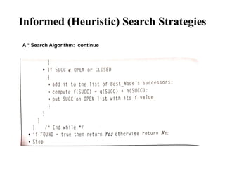
- 42. Informed (Heuristic) Search Strategies A * Search Algorithm: continue
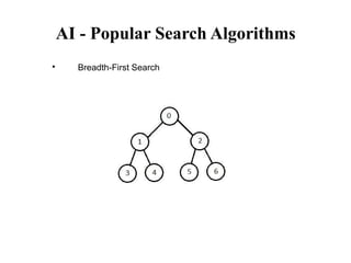
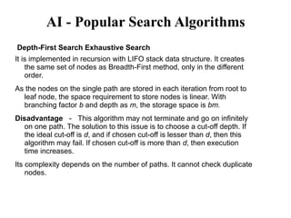
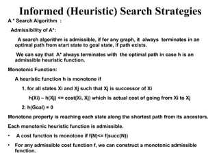
- 43. Informed (Heuristic) Search Strategies A * Search Algorithm example: Let us consider eight puzzle problem and solve it by A* algorithm. Let define the evaluation function as: f(X) = g(X) + h(X), where [ f(startstate)= 0 + 4 = 4 ] h(X) = the number of tiles not in their goal position in a given state X g(X) = depth of node X in the search tree Start state Goal State 3 7 6 5 1 2 4 8 5 3 6 7 2 4 1 8
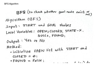
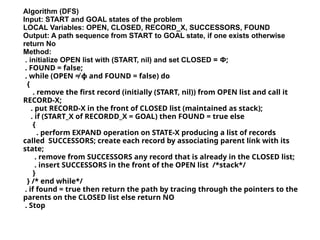
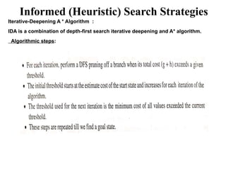
- 44. Informed (Heuristic) Search Strategies A * Search Algorithm example: Let us consider eight puzzle problem and solve it by A* algorithm. Let define the evaluation function as: f(X) = g(X) + h(X), where [ f(startstate)= 0 + 4 ] h(X) = the number of tiles not in their goal position in a given state X = 4 g(X) = depth of node X in the search tree [for start node = 0] Start state Goal State 3 7 6 5 1 2 4 8 5 3 6 7 2 4 1 8
- 45. Informed (Heuristic) Search Strategies A * Search Algorithm example : search tree
- 46. Informed (Heuristic) Search Strategies A * Search Algorithm : Note: The quality of the solution depends on the heuristic function. Hence, the heuristic function used above may not be better for harder eight-puzzle problems. The above eight-puzzle problem can not be solved by simple heuristic function given above. We need to find the better heuristic function by estimating the h() value properly. Let we keep function g(X) as same and function h(X) modified as: h(X) = the sum of the distances of the tiles ( 1 to 8) from their goal position in a given state X. 5 3 6 7 2 4 1 8 3 5 1 2 7 4 8 6 Start state Goal state h(start state)= m(1) + m(2) + m(3) + m(4) + m(5) + m(6) + m(7) + m(8) = 3 + 2 + 1 + 0 + 1 + 2 + 2 + 1 = 12
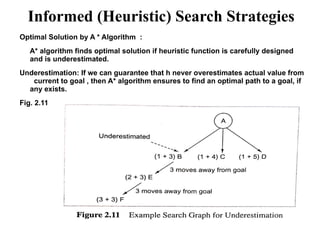
- 47. Informed (Heuristic) Search Strategies Optimal Solution by A * Algorithm : A* algorithm finds optimal solution if heuristic function is carefully designed and is underestimated. Underestimation: If we can guarantee that h never overestimates actual value from current to goal , then A* algorithm ensures to find an optimal path to a goal, if any exists. Fig. 2.11
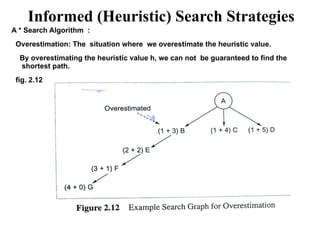
- 48. Informed (Heuristic) Search Strategies A * Search Algorithm : Overestimation: The situation where we overestimate the heuristic value. By overestimating the heuristic value h, we can not be guaranteed to find the shortest path. fig. 2.12
- 49. Informed (Heuristic) Search Strategies A * Search Algorithm : Admissibility of A*: A search algorithm is admissible, if for any graph, it always terminates in an optimal path from start state to goal state, if path exists. We can say that A* always terminates with the optimal path in case h is an admissible heuristic function. Monotonic Function: A heuristic function h is monotone if 1. for all states Xi and Xj such that Xj is successor of Xi h(Xi) ÔÇô h(Xj) <= cost(Xi, Xj) which is actual cost of going from Xi to Xj 2. h(Goal) = 0 Monotone property is reaching each state along the shortest path from its ancestors. Each monotonic heuristic function is admissible. ÔÇó A cost function is monotone if f(N)<= f(succ(N)) ÔÇó For any admissible cost function f, we can construct a monotonic admissible function.
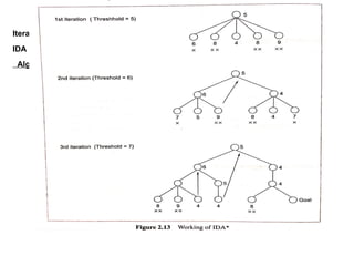
- 50. Informed (Heuristic) Search Strategies Iterative-Deepening A * Algorithm : IDA is a combination of depth-first search iterative deepening and A* algorithm. Algorithmic steps:
- 51. Informed (Heuristic) Search Strategies Iterative-Deepening A * Algorithm : IDA is a combination of depth-first search iterative deepening and A* algorithm. Algorithmic steps:
- 52. Informed (Heuristic) Search Strategies ´ü¼ Greedy Best First Search It expands the node that is estimated to be closest to goal. It expands nodes based on f(n) = h(n). It is implemented using priority queue. Disadvantage ´╝ì It can get stuck in loops. It is not optimal.
- 53. Local Search Algorithms Disadvantage ´╝ì This algorithm is neither complete, nor optimal.
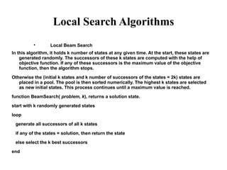
- 54. Local Search Algorithms ´ü¼ Local Beam Search In this algorithm, it holds k number of states at any given time. At the start, these states are generated randomly. The successors of these k states are computed with the help of objective function. If any of these successors is the maximum value of the objective function, then the algorithm stops. Otherwise the (initial k states and k number of successors of the states = 2k) states are placed in a pool. The pool is then sorted numerically. The highest k states are selected as new initial states. This process continues until a maximum value is reached. function BeamSearch( problem, k), returns a solution state. start with k randomly generated states loop generate all successors of all k states if any of the states = solution, then return the state else select the k best successors end
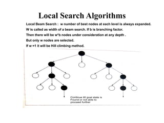
- 55. Local Search Algorithms Local Beam Search : w number of best nodes at each level is always expanded. W is called as width of a beam search. If b is branching factor. Then there will be w*b nodes under consideration at any depth . But only w nodes are selected. If w =1 it will be Hill climbing method. example