Andrew Goldberg. An Efficient Point-to¿CPoint Shortest Path Algorithm
- 1. Point-to-Point Shortest Path Algorithms with Preprocessing Andrew V. Goldberg Microsoft Research ¿C Silicon Valley www.research.microsoft.com/í½goldberg/ Joint with Haim Kaplan and Renato Werneck
- 2. Einstein Quote Everything should be made as simple as possible, but not simpler SP with preprocessing 1
- 3. Shortest Path Problem Variants ? Nonnegative and arbitrary arc lengths. ? Point to point, single source, all pairs. ? Directed and undirected. Here we study ? Point to point, nonnegative length, directed problem. ? Allow preprocessing with limited (linear) space. Many applications, both directly and as a subroutine. SP with preprocessing 2
- 4. Shortest Path Problem Input: Directed graph G = (V, A), nonnegative length function : A í· R+ , origin s í╩ V , destination t í╩ V . Preprocessing: Limited space to store results. Query: Find a shortest path from s to t. Interested in exact algorithms that search a (small) subgraph. Related work: reach-based routing [Gutman 04], hierarchi- cal decomposition [Schultz, Wagner & Weihe 02], [Sanders & Schultes 05, 06], geometric pruning [Wagner & Willhalm 03], arc ?ags [Lauther 04], [Kíºhler, Míºhring & Schilling 05], [Míºhring o o o et al. 06]. SP with preprocessing 3
- 5. Motivating Application Driving directions ? Run on servers and small devices. ? Typical production codes ? Use base graph or other heuristics based on road cate- gories; needs hand-tuning. ? Runs (bidirectional) Dijkstra or A? with Euclidean bounds on í░patchedí▒ graph. ? Non-exact and no performance guarantee. ? We are interested in exact and very e?cient algorithms. ? New results ?nding their way into products. SP with preprocessing 4
- 6. Outline ? Scanning method and Dijkstraí»s algorithm. ? Bidirectional Dijkstraí»s algorithm. ? A? search. ? ALT Algorithm ? De?nition of reach ? Reach-based algorithm ? Reach for A? SP with preprocessing 5
- 7. Scanning Method ? For each vertex v maintain its distance label ds(v) and status S(v) í╩ {unreached, labeled, scanned}. ? Unreached vertices have ds(v) = íÌ. ? If ds(v) decreases, v becomes labeled. ? To scan a labeled vertex v, for each arc (v, w), if ds(w) > ds(v) + (v, w) set ds (w) = ds(v) + (v, w). ? Initially for all vertices are unreached. ? Start by decreasing ds(s) to 0. ? While there are labeled vertices, pick one and scan it. ? Di?erent selection rules lead to di?erent algorithms. SP with preprocessing 6
- 8. Dijkstraí»s Algorithm [Dijkstra 1959], [Dantzig 1963]. ? At each step scan a labeled vertex with the minimum label. ? Stop when t is selected for scanning. Work almost linear in the visited subgraph size. Reverse Algorithm: Run algorithm from t in the graph with all arcs reversed, stop when t is selected for scanning. Bidirectional Algorithm ? Run forward Dijkstra from s and backward from t. ? Maintain ?, the length of the shortest path seen: when scan- ning an arc (v, w) such that w has been scanned in the other direction, check if the corresponding s-t path improves ?. ? Stop when about to scan a vertex x scanned in the other direction. ? Output ? and the corresponding path. SP with preprocessing 7
- 9. Bidirectional Algorithm: Pitfalls The algorithm is not as simple as it looks. 2 a 5 b 2 s t 5 x 5 The searches meat at x, but x is not on the shortest path. SP with preprocessing 8
- 10. Example Graph 1.6M vertices, 3.8M arcs, travel time metric. SP with preprocessing 9
- 11. Dijkstraí»s Algorithm Searched area SP with preprocessing 10
- 12. Bidirectional Algorithm forward search/ reverse search SP with preprocessing 11
- 13. A? Search [Doran 67], [Hart, Nilsson & Raphael 68] Motivated by large search spaces (e.g., game graphs). Similar to Dijkstraí»s algorithm but: ? Domain-speci?c estimates ªðt(v) on dist(v, t) (potentials). ? At each step pick a labeled vertex with the minimum k(v) = ds(v) + ªðt(v). Best estimate of path length. ? In general, optimality is not guaranteed. 1 11 00 111111 000000 2 1 0 1111111 3 11 00 111111 0 4 1 0 00000000000000000 111111 0 1111111 0000000 11 00 111111 000000 1 0 11 00 1 0 1111111 0000000 11 00 111111 000000 1 0 11 00 1 0 1111111 0000000 111111 000000 0 4 111111 000000 3 2 1111111 0000000 1 5 1111111 0000000 11111111111 00000000000 111111 000000 1 0 11111111111 00000000000 1111111 0000000 1 0 1111111 0000000 1 0 11111111111 00000000000 1 0 1111111 0000000 11111111111 00000000000 1111111 0000000 0 11111111111 00000000000 11111111111 00000000000 1111111 0000000 1111111 0000000 1 0 1 0 11 00 111111 1 0 00000000000 111111 0 11 00 1 0 6 2 1 SP with preprocessing 12
- 14. Feasibility and Optimality Potential transformation: Replace (v, w) by ªðt (v, w) = (v, w) ? ªðt(v) + ªðt(w) (reduced costs). Fact: Problems de?ned by and ªðt are equivalent. De?nition: ªðt is feasible if ?(v, w) í╩ A, the reduced costs are nonnegative. (Estimates are í░locally consistentí▒.) Optimality: If ªðt is feasible, the A? search is equivalent to Dijk- straí»s algorithm on transformed network, which has nonnegative arc lengths. A? search ?nds an optimal path. Di?erent order of vertex scans, di?erent subgraph searched. Fact: If ªðt is feasible and ªðt(t) = 0, then ªðt gives lower bounds on distances to t. SP with preprocessing 13
- 15. Computing Lower Bounds Euclidean bounds: [folklore], [Pohl 71], [Sedgewick & Vitter 86]. For graph embedded in a metric space, use Euclidean distance. Limited applicability, not very good for driving directions. We use triangle inequality a000 1111111111111 0000000000000 111 b 11111111111111 00000000000000 111 000 11 11111111111111 00 00000000000000 1111111111111 0000000000000 111 000 1 0 111 000 11 11111111111111 00 00000000000000 1111111111111 0000000000000 111 000 1 0 111 000 1111111111111 0000000000000 111 000 11111111111111 00000000000000 1111111111111 0000000000000 111 000 111 000 11111111111111 00000000000000 111 000 1 0 11 00 1111111111111 0000000000000 111 000 11111111111111 00000000000000 11111111111111 00000000000000 1 0 1 0 11 00 11 00 v w dist(v, w) í¦ dist(v, b)?dist(w, b); dist(v, w) í¦ dist(a, w)?dist(a, v). SP with preprocessing 14
- 16. Lower Bounds (cont.) Maximum (minimum, average) of feasible potentials is feasible. ? Select landmarks (a small number). ? For all vertices, precompute distances to and from each land- mark. ? For each s, t, use max of the corresponding lower bounds for ªðt(v). Why this works well (when it does) a s x y t ªðt (x, y) = 0 SP with preprocessing 15
- 17. Bidirectional Lowerbounding Forward reduced costs: ªðt (v, w) = (v, w) ? ªðt(v) + ªðt(w). Reverse reduced costs: ªðs (v, w) = (v, w) + ªðs(v) ? ªðs(w). Whatí»s the problem? SP with preprocessing 16
- 18. Bidirectional Lowerbounding Forward reduced costs: ªðt (v, w) = (v, w) ? ªðt(v) + ªðt(w). Reverse reduced costs: ªðs (v, w) = (v, w) + ªðs(v) ? ªðs(w). Fact: ªðt and ªðs give the same reduced costs i? ªðs + ªðt = const. [Ikeda et at. 94]: use ps(v) = ªðs(v)?ªðt(v) and pt (v) = ?ps(v). 2 Other solutions possible. Easy to loose correctness. ALT algorithms use A? search and landmark-based lower bounds. SP with preprocessing 17
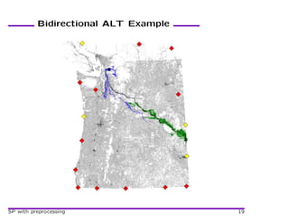
- 19. Landmark Selection Preprocessing ? Random selection is fast. ? Many heuristics ?nd better landmarks. ? Local search can ?nd a good subset of candidate landmarks. ? We use a heuristic with local search. Preprocessing/query trade-o?. Query ? For a speci?c s, t pair, only some landmarks are useful. ? Use only active landmarks that give best bounds on dist(s, t). ? If needed, dynamically add active landmarks (good for the search frontier). Allows using many landmarks with small time overhead. SP with preprocessing 18
- 20. Bidirectional ALT Example SP with preprocessing 19
- 21. Experimental Results Northwest (1.6M vertices), random queries, 16 landmarks. preprocessing query method minutes MB avgscan maxscan ms Bidirectional Dijkstra í¬ 28 518 723 1 197 607 340.74 ALT 4 132 16 276 150 389 12.05 SP with preprocessing 20
- 22. Related Systems Work Network delay estimation: Use delays to beacons to estimate arbitrary node delays. E.g., IDMaps [Francis et al. 01]. Theoretical analysis [Kleinberg, Slivkins & Wexler 04]: for ran- dom beacons and bounded doubling dimension graphs, get good bounds for most node pairs. Good bounds are not enough to prove bounds on ALT. SP with preprocessing 21
- 23. Reach Intuition Identify local intersections and prune them when searching far from s and t. SP with preprocessing 22
- 24. Reaches [Gutman 04] ? Consider a vertex v that splits a path P into P1 and P2. rP (v) = min( (P1), (P2)). ? r(v) = maxP (rP (v)) over all shortest paths P through v. Using reaches to prune Dijkstra: LB(w,t) d(s,v) v w s t If r(w) < min(d(v) + (v, w), LB(w, t)) then prune w. SP with preprocessing 23
- 25. Obtaining Lower Bounds Can use landmark lower bounds if available. Bidirectional search gives implicit bounds (Rt below). LB(w,t) d(s,v) v w s Rt t Reach-based query algorithm is Dijkstraí»s algorithm with prun- ing based on reaches. Given a lower-bound subroutine, a small change to Dijkstraí»s algorithm. SP with preprocessing 24
- 26. Computing Reaches ? A natural exact computation uses all-pairs shortest paths. ? Overnight for 0.3M vertex graph, years for 30M vertex graph. ? Have a heuristic improvement, but it is not fast enough. ? Can use reach upper bounds for query search pruning. Iterative approximation algorithm: [Gutman 04] ? Use partial shortest path trees of depth O( ) to bound reaches of vertices v with r(v) < . ? Delete vertices with bounded reaches, add penalties. ? Increase and repeat. Query time does not increase much; preprocessing faster but still not fast enough. SP with preprocessing 25
- 27. Reach Algorithm SP with preprocessing 26
- 28. Experimental Results Northwest (1.6M vertices), random queries, 16 landmarks. preprocessing query method minutes MB avgscan maxscan ms Bidirectional Dijkstra í¬ 28 518 723 1 197 607 340.74 ALT 4 132 16 276 150 389 12.05 Reach 1 100 34 53 888 106 288 30.61 SP with preprocessing 27
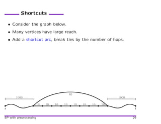
- 29. Shortcuts ? Consider the graph below. ? Many vertices have large reach. 1000 1000 10 10 10 10 10 10 10 10 s 1000 1010 1020 1030 1040 1030 1020 1010 1000 t SP with preprocessing 28
- 30. Shortcuts ? Consider the graph below. ? Many vertices have large reach. ? Add a shortcut arc, break ties by the number of hops. 80 1000 1000 10 10 10 10 10 10 10 10 s t SP with preprocessing 29
- 31. Shortcuts ? Consider the graph below. ? Many vertices have large reach. ? Add a shortcut arc, break ties by the number of hops. ? Reaches decrease. s 1000 60 50 40 30 40 50 60 1000 t SP with preprocessing 30
- 32. Shortcuts ? Consider the graph below. ? Many vertices have large reach. ? Add a shortcut arc, break ties by the number of hops. ? Reaches decrease. ? Repeat. s 1000 20 10 20 30 20 10 20 1000 t SP with preprocessing 31
- 33. Shortcuts ? Consider the graph below. ? Many vertices have large reach. ? Add a shortcut arc, break ties by the number of hops. ? Reaches decrease. ? Repeat. ? A small number of shortcuts can greatly decrease many reaches. s 1000 0 10 0 30 0 10 0 1000 t SP with preprocessing 32
- 34. Shortcuts [Sanders & Schultes 05, 06]: similar idea in hierarchy-based al- gorithm; similar performance. ? During preprocessing we shortcut small-degree vertices every time is updated. ? Shortcut replaces a vertex by a clique on its neighbors. ? A constant number of arcs is added for each deleted vertex. ? Shortcuts greatly speed up preprocessing. ? Shortcuts speed up queries. SP with preprocessing 33
- 35. Reach with Shortcuts SP with preprocessing 34
- 36. Experimental Results Northwest (1.6M vertices), random queries, 16 landmarks. preprocessing query method minutes MB avgscan maxscan ms Bidirectional Dijkstra í¬ 28 518 723 1 197 607 340.74 ALT 4 132 16 276 150 389 12.05 Reach 1 100 34 53 888 106 288 30.61 Reach+Short 17 100 2 804 5 877 2.39 SP with preprocessing 35
- 37. Reaches and ALT ? ALT computes transformed and original distances. ? ALT can be combined with reach pruning. ? Careful: Implicit lower bounds do not work, but landmark lower bounds do. ? Shortcuts do not a?ect landmark distances and bounds. SP with preprocessing 36
- 38. Reach with Shortcuts and ALT SP with preprocessing 37
- 39. Experimental Results Northwest (1.6M vertices), random queries, 16 landmarks. preprocessing query method minutes MB avgscan maxscan ms Bidirectional Dijkstra í¬ 28 518 723 1 197 607 340.74 ALT 4 132 16 276 150 389 12.05 Reach 1 100 34 53 888 106 288 30.61 Reach+Short 17 100 2 804 5 877 2.39 Reach+Short+ALT 21 204 367 1 513 0.73 SP with preprocessing 38
- 40. Further Improvements ? Improved locality (sort by reach). ? For RE, factor of 3 ? 12 improvement for preprocessing and factor of 2 ? 4 for query times. ? Reach-aware landmarks: time/space trade-o?. ? Idea: maintain landmark distances for a small fraction of high-reach vertices only. ? Can use more landmarks and improve both time and space. Practical even for large (USA, Europe) graphs ? íÍ 1 ms. query time on a server. ? íÍ 5sec. query time on a Pocket PC with 2GB ?ash card. ? Better for local queries. SP with preprocessing 39
- 41. The USA Graph USA: 24M vertices, 58M arcs, time metric, random queries. preprocessing query method min KB avgscan maxscan ms Dijkstra í¬ 536 11 808 864 í¬ 5 440.49 ALT(16) 17.6 2 563 187 968 2 183 718 295.44 Reach impractical Reach+Short 27.9 893 2 405 4 813 1.77 Reach+Short+ALT(16,1) 45.5 3 032 592 2 668 0.80 Reach+Short+ALT(64,16) 113.9 1 579 538 2 534 0.86 SP with preprocessing 40
- 42. The USA Graph USA: 24M vertices, 58M arcs, distance metric, random queries. preprocessing query method min KB avgscan maxscan ms Dijkstra í¬ 536 11 782 104 í¬ 4 576.02 ALT(16) 15.2 2 417 276 195 2 910 133 410.73 Reach impractical Reach+Short 46.4 918 7 311 13 886 5.78 Reach+Short+ALT(16,1) 61.5 2 923 905 5 510 1.41 Reach+Short+ALT(64,16) 120.5 1 575 670 3 499 1.22 SP with preprocessing 41
- 43. Europe Graph Europe: 18M vertices, 43M arcs, time metric, random queries. preprocessing query method min KB avgscan maxscan ms Dijkstra í¬ 393 8 984 289 í¬ 4 365.81 ALT(16) 12.5 1 597 82 348 993 015 120.09 Reach impractical Reach+Short 45.1 648 4 371 8 486 3.06 Reach+Short+ALT(16,1) 57.7 1 869 714 3 387 0.89 Reach+Short+ALT(64,16) 102.6 1 037 610 2 998 0.91 SP with preprocessing 42
- 44. Grid Graphs Grid with uniform random lengths (0.5M vertices), 16 landmarks. No highway structure. preprocessing query method min MB avgscan maxscan ms Bidirectional Dijkstra í¬ 18.0 174 150 416 925 160.14 ALT 0.26 96.6 6 057 65 664 6.28 Reach+Short 7.77 27.7 6 458 10 049 4.75 Reach+Short+ALT(16,1) 8.03 106.3 558 3 189 0.89 Reach+Short+ALT(64,16) 9.14 49.2 2 823 3 711 2.67 Reach preprocessing expensive, but helps queries. (64,16) signi?cantly slower that (16,1). SP with preprocessing 43
- 45. Demo SP with preprocessing 44
- 46. Concluding Remarks ? Our heuristics work well on road networks. ? Recent improvements: [Bast et al. 07, Geisberger et al. 08]. ? How to select good shortcuts? (Road networks/grids.) ? For which classes of graphs do these techniques work? ? Need theoretical analysis for interesting graph classes. ? Interesting problems related to reach, e.g. ? Is exact reach as hard as all-pairs shortest paths? ? ? Constant-ratio upper bounds on reaches in O(m) time. ? Dynamic graphs (real-time tra?c). SP with preprocessing 45


![Shortest Path Problem
Input: Directed graph G = (V, A), nonnegative length function
: A í· R+ , origin s í╩ V , destination t í╩ V .
Preprocessing: Limited space to store results.
Query: Find a shortest path from s to t.
Interested in exact algorithms that search a (small) subgraph.
Related work: reach-based routing [Gutman 04], hierarchi-
cal decomposition [Schultz, Wagner & Weihe 02], [Sanders &
Schultes 05, 06], geometric pruning [Wagner & Willhalm 03], arc
?ags [Lauther 04], [Kíºhler, Míºhring & Schilling 05], [Míºhring
o o o
et al. 06].
SP with preprocessing 3](https://image.slidesharecdn.com/20080601ppspgoldberg-100622234412-phpapp01/85/Andrew-Goldberg-An-Efficient-Point-to-Point-Shortest-Path-Algorithm-4-320.jpg)


![Dijkstraí»s Algorithm
[Dijkstra 1959], [Dantzig 1963].
? At each step scan a labeled vertex with the minimum label.
? Stop when t is selected for scanning.
Work almost linear in the visited subgraph size.
Reverse Algorithm: Run algorithm from t in the graph with all
arcs reversed, stop when t is selected for scanning.
Bidirectional Algorithm
? Run forward Dijkstra from s and backward from t.
? Maintain ?, the length of the shortest path seen: when scan-
ning an arc (v, w) such that w has been scanned in the other
direction, check if the corresponding s-t path improves ?.
? Stop when about to scan a vertex x scanned in the other
direction.
? Output ? and the corresponding path.
SP with preprocessing 7](https://image.slidesharecdn.com/20080601ppspgoldberg-100622234412-phpapp01/85/Andrew-Goldberg-An-Efficient-Point-to-Point-Shortest-Path-Algorithm-8-320.jpg)


![A? Search
[Doran 67], [Hart, Nilsson & Raphael 68]
Motivated by large search spaces (e.g., game graphs).
Similar to Dijkstraí»s algorithm but:
? Domain-speci?c estimates ªðt(v) on dist(v, t) (potentials).
? At each step pick a labeled vertex with the minimum k(v) =
ds(v) + ªðt(v).
Best estimate of path length.
? In general, optimality is not guaranteed.
1
11
00
111111
000000
2
1
0
1111111
3
11
00
111111
0
4
1
0
00000000000000000
111111
0 1111111
0000000
11
00
111111
000000 1
0 11
00 1
0
1111111
0000000
11
00
111111
000000 1
0 11
00 1
0
1111111
0000000
111111
000000
0 4
111111
000000 3 2 1111111
0000000
1 5
1111111
0000000
11111111111
00000000000
111111
000000
1
0
11111111111
00000000000 1111111
0000000
1
0
1111111
0000000
1
0
11111111111
00000000000 1
0
1111111
0000000
11111111111
00000000000 1111111
0000000
0
11111111111
00000000000
11111111111
00000000000 1111111
0000000
1111111
0000000
1
0
1
0 11
00
111111 1
0
00000000000
111111
0
11
00 1
0
6 2 1
SP with preprocessing 12](https://image.slidesharecdn.com/20080601ppspgoldberg-100622234412-phpapp01/85/Andrew-Goldberg-An-Efficient-Point-to-Point-Shortest-Path-Algorithm-13-320.jpg)

![Computing Lower Bounds
Euclidean bounds:
[folklore], [Pohl 71], [Sedgewick & Vitter 86].
For graph embedded in a metric space, use Euclidean distance.
Limited applicability, not very good for driving directions.
We use triangle inequality
a000
1111111111111
0000000000000
111
b
11111111111111
00000000000000
111
000
11 11111111111111
00 00000000000000
1111111111111
0000000000000
111
000 1
0
111
000
11 11111111111111
00 00000000000000
1111111111111
0000000000000
111
000 1
0
111
000
1111111111111
0000000000000
111
000
11111111111111
00000000000000
1111111111111
0000000000000
111
000 111
000
11111111111111
00000000000000
111
000
1
0 11
00
1111111111111
0000000000000
111
000
11111111111111
00000000000000
11111111111111
00000000000000
1
0
1
0
11
00
11
00
v w
dist(v, w) í¦ dist(v, b)?dist(w, b); dist(v, w) í¦ dist(a, w)?dist(a, v).
SP with preprocessing 14](https://image.slidesharecdn.com/20080601ppspgoldberg-100622234412-phpapp01/85/Andrew-Goldberg-An-Efficient-Point-to-Point-Shortest-Path-Algorithm-15-320.jpg)


![Bidirectional Lowerbounding
Forward reduced costs: ªðt (v, w) = (v, w) ? ªðt(v) + ªðt(w).
Reverse reduced costs: ªðs (v, w) = (v, w) + ªðs(v) ? ªðs(w).
Fact: ªðt and ªðs give the same reduced costs i? ªðs + ªðt = const.
[Ikeda et at. 94]: use ps(v) = ªðs(v)?ªðt(v) and pt (v) = ?ps(v).
2
Other solutions possible. Easy to loose correctness.
ALT algorithms use A? search and landmark-based lower bounds.
SP with preprocessing 17](https://image.slidesharecdn.com/20080601ppspgoldberg-100622234412-phpapp01/85/Andrew-Goldberg-An-Efficient-Point-to-Point-Shortest-Path-Algorithm-18-320.jpg)


![Related Systems Work
Network delay estimation:
Use delays to beacons to estimate arbitrary node delays.
E.g., IDMaps [Francis et al. 01].
Theoretical analysis [Kleinberg, Slivkins & Wexler 04]: for ran-
dom beacons and bounded doubling dimension graphs, get good
bounds for most node pairs.
Good bounds are not enough to prove bounds on ALT.
SP with preprocessing 21](https://image.slidesharecdn.com/20080601ppspgoldberg-100622234412-phpapp01/85/Andrew-Goldberg-An-Efficient-Point-to-Point-Shortest-Path-Algorithm-22-320.jpg)

![Reaches
[Gutman 04]
? Consider a vertex v that splits a path P into P1 and P2.
rP (v) = min( (P1), (P2)).
? r(v) = maxP (rP (v)) over all shortest paths P through v.
Using reaches to prune Dijkstra:
LB(w,t)
d(s,v) v w
s t
If r(w) < min(d(v) + (v, w), LB(w, t)) then prune w.
SP with preprocessing 23](https://image.slidesharecdn.com/20080601ppspgoldberg-100622234412-phpapp01/85/Andrew-Goldberg-An-Efficient-Point-to-Point-Shortest-Path-Algorithm-24-320.jpg)

![Computing Reaches
? A natural exact computation uses all-pairs shortest paths.
? Overnight for 0.3M vertex graph, years for 30M vertex graph.
? Have a heuristic improvement, but it is not fast enough.
? Can use reach upper bounds for query search pruning.
Iterative approximation algorithm: [Gutman 04]
? Use partial shortest path trees of depth O( ) to bound reaches
of vertices v with r(v) < .
? Delete vertices with bounded reaches, add penalties.
? Increase and repeat.
Query time does not increase much; preprocessing faster but still
not fast enough.
SP with preprocessing 25](https://image.slidesharecdn.com/20080601ppspgoldberg-100622234412-phpapp01/85/Andrew-Goldberg-An-Efficient-Point-to-Point-Shortest-Path-Algorithm-26-320.jpg)


![Shortcuts
[Sanders & Schultes 05, 06]: similar idea in hierarchy-based al-
gorithm; similar performance.
? During preprocessing we shortcut small-degree vertices every
time is updated.
? Shortcut replaces a vertex by a clique on its neighbors.
? A constant number of arcs is added for each deleted vertex.
? Shortcuts greatly speed up preprocessing.
? Shortcuts speed up queries.
SP with preprocessing 33](https://image.slidesharecdn.com/20080601ppspgoldberg-100622234412-phpapp01/85/Andrew-Goldberg-An-Efficient-Point-to-Point-Shortest-Path-Algorithm-34-320.jpg)


![Concluding Remarks
? Our heuristics work well on road networks.
? Recent improvements: [Bast et al. 07, Geisberger et al. 08].
? How to select good shortcuts? (Road networks/grids.)
? For which classes of graphs do these techniques work?
? Need theoretical analysis for interesting graph classes.
? Interesting problems related to reach, e.g.
? Is exact reach as hard as all-pairs shortest paths?
?
? Constant-ratio upper bounds on reaches in O(m) time.
? Dynamic graphs (real-time tra?c).
SP with preprocessing 45](https://image.slidesharecdn.com/20080601ppspgoldberg-100622234412-phpapp01/85/Andrew-Goldberg-An-Efficient-Point-to-Point-Shortest-Path-Algorithm-46-320.jpg)