Global network structure of dominance hierarchy of ant workersAntnet slides-slideshare
- 1. Dominance hierarchy of worker ants as directed networks Hiroyuki Shimoji (Univ. Ryukyus, Japan & Univ. Tokyo, Japan) Masato S. Abe (Univ. Tokyo) Kazuki Tsuji (Univ. Ryukyus) Naoki Masuda (University of Bristol, UK) Ref: Shimoji, Abe, Tsuji & Masuda, J. R. Soc. Interface, in press (2014); arXiv:1407.4277; data available online
- 2. Dominance hierarchy ŌĆó Pecking order of hens (Schjelderup-Ebbe, 1922) ŌĆó Automise the access to food/mates/space/shelter ŌĆó Reduce aggregation ŌĆó Keep workers to work for the colonyŌĆÖs benefit Thorleif Schjelderup-Ebbe (1894-1976) - Ō£ö’ĖÄ Ō£ö’ĖÄ Ō£ö’ĖÄ Ō£ö’ĖÄ Ō£ö’ĖÄ - Ō£ö’ĖÄ Ō£ö’ĖÄ Ō£ö’ĖÄ Ō£ö’ĖÄ - Ō£ö’ĖÄ Ō£ö’ĖÄ Ō£ö’ĖÄ - Ō£ö’ĖÄ Ō£ö’ĖÄ - Ō£ö’ĖÄ - self peer Icon and picture from Freepik.com and Wikipedia
- 3. Dominance hierarchy as network ŌĆó Most studies have focused on ŌĆó How close data are to ŌĆ£linearŌĆØ hierarchy ŌĆó How to rank individuals in a group ŌĆó Small groups ŌĆó Network analysis of dominance hierarchy has been surprisingly rare. ŌĆó Some recent work as undirected networks ŌĆó Triad census (Shizuka & McDonald, 2012)
- 4. Diacamma sp. ŌĆó Monogynous ŌĆó A colony contains at most one (functional, not morphological) queen. ŌĆó 20-300 workers, i.e., ŌĆ£largeŌĆØ groups ŌĆó Suitable for observing behaviour: ŌĆó Large body size ŌĆó Many previous studies
- 5. nest marked workers aggressive behaviour (bite and jerk) = directed link Photos by H. Shimoji
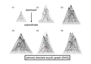
- 6. ŌĆó 4 days of observation (5 h/day) colony # nodes avg deg # bidir links C1 20 2.9 0/29 C2 32 3.4 0/55 C3 48 5.6 0/134 C4 70 4.5 0/158 C5 56 4.8 2/133 C6 64 4.3 0/137 ŌĆ£largeŌĆØ network (almost) acyclic?sparse
- 7. (almost) directed acyclic graph (DAG) dominant subordinate
- 8. A B C D E F G A B C D E F G 6 1 4 6 8 5 5 5 2 1 2 2 1 1 15 1 11 1 4 2 DAG hierarchy is not trivial 1. In large groups, linear hierarchy is often violated. data from Appleby, Animal Behaviour, 1983 winner dominant dominant red deer stags A B C D E F G A B C D E F G Ō£ō Ō£ō Ō£ō Ō£ō Ō£ō Ō£ō Ō£ō Ō£ō Ō£ō Ō£ō Ō£ō Ō£ō Ō£ō A F G E B D C A F G E B D C Ō£ō Ō£ō Ō£ō Ō£ō Ō£ō Ō£ō Ō£ō Ō£ō Ō£ō Ō£ō Ō£ō Ō£ō Ō£ō subordinatesubordinateloser
- 9. DAG hierarchy is not trivial 2. There are various DAGs. ŌĆó Variation in link density ŌĆó Even for a fixed link density, various DAGs linear tournament arborescence
- 10. Quantifications of DAGs (link weight ignored) 1. Reversibility (Corominas-Murtra, Rodr├Łguez-Caso, Go├▒i, Sol├®, 2010) ŌĆó Information necessary to reversely travel to the most dominant nodes 2. Hierarchy (their 2011) ╬Į Ōłł [-1, 1] ŌĆó ╬Į = 0 Ō¤║ lack of hierarchy in either direction
- 11. Quantifications of DAGs (cntŌĆÖd) 3. Global reaching centrality (Mones, Vicsek, Vicsek, 2012): ŌĆó Large GRC Ō¤║ directed paths starting from a small fraction of nodes reach a majority of nodes ŌĆó Directed star: GRC = 1 ŌĆó 0 Ōēż GRC Ōēż 1 4. Network motif (Milo et al. 2002) GRC = 1 N 1 NX i=1 [Cmax R CR(i)] , where Cmax R = max i CR(i) CR(i) : local reaching centrality of node i
- 12. Null model networks ŌĆó Randomised DAGs (Go├▒i, Corominas-Murtra, Sol├®, Rodr├Łguez-Caso, 2010) ŌĆó In-degree and out-degree of each node are fixed. ŌĆó Thinned linear tournament (= cascade model by J. E. Cohen & C. M. Newman, 1985) ŌĆó Number of links matched ŌĆó Does not conserve in/out- degree of each node ŌĆó Then, calculate the Z score: e.g., p=0.6 Z = GRCobserved ┬Ąnull(GRC) null(GRC)
- 13. Ō£ö’ĖÄ Similar results for link-reversed dominance networks colony Reversibility (H Ōēź 0)Reversibility (H Ōēź 0)Reversibility (H Ōēź 0) Hierarchy (0 Ōēż ╬Į Ōēż 1)Hierarchy (0 Ōēż ╬Į Ōēż 1)Hierarchy (0 Ōēż ╬Į Ōēż 1) GRC (0 Ōēż GRC Ōēż 1)GRC (0 Ōēż GRC Ōēż 1)GRC (0 Ōēż GRC Ōēż 1) colony Value Thinned tournament Random DAG Value Thinned tournament Random DAG Value Thinned tournament Random DAG C1 0.28 -2.36* - 0.59 3.68** -0.33 0.94 4.45** 1.01 C2 1.41 1.86 1.76 0.14 1.05 -1.70 0.71 2.72** -2.11* C3 1.73 0.24 2.33* 0.31 3.32** 0.05 0.88 4.93** -1.40 C4 1.33 -0.36 -1.33 0.32 3.90** -1.08 0.96 6.60** 1.66 C5 2.37 4.98** 0.20 0.28 3.15** 0.74 0.86 4.82** -0.89 C6 2.02 4.09** 1.69 0.14 1.72 0.66 0.82 4.54** -0.64 *: p<0.05; **: p<0.01
- 14. Ō£ö’ĖÄ Similar results for link-reversed dominance networks *: p<0.05; **: p<0.01
- 15. LetŌĆÖs look at the degree attacked by 2 workers (in-degree = 2) attacks 3 workers (out-degree = 3) Photo by H. Shimoji
- 16. Only the out-degree is heterogeneously distributed (CV = 1.9-3.5)
- 19. Out-strength out-strength = 8 1 4 3 5 3 link weight = # observed aggressive behaviour Photo by H. Shimoji
- 20. The top ranker is often not the most frequent attackers. Out-strength vs workerŌĆÖs rank
- 21. Summary of the observations ŌĆó Empirical dominance networks are close to random DAGs. ŌĆó Similar to citation networks (Karrer & Newman, PRL, PRE 2009) ŌĆó Not close to the thinned linear tournament ŌĆó Sparse ŌĆó Out-degree: heterogeneous, in-degree: not so much ŌĆó Most aggressive workers are near the top (but not necessarily the very top) of the hierarchy.
- 22. Discussion ŌĆó How is the link density regulated? ŌĆó Cost of attacking ŌĆó Benefit of keeping hierarchy: workers work for the colony (so-called indirect fitness) ŌĆó Why (evolutionarily) does the DAG-like dominance hierarchy form? ŌĆó For high rankers, more chances to reproduce (direct fitness) ŌĆó For low rankers in the bottom of hierarchy, why? ŌĆó Why does the top ranker limit the number of direct subordinates? ŌĆó Generative models? Ref: Shimoji, Abe, Tsuji & Masuda, J. R. Soc. Interface, in press (2014)
- 23. Discussion (cntŌĆÖd) ŌĆó Linearity is not detected by previous methods due to sparseness. colony hŌĆÖ P(hŌĆÖ) ŌĆÖ) ttri P(ttri) C1 0.21 0.18 1 0.39 C2 0.12 0.23 1 0.23 C3 0.13 0.0003 1 0.001 C4 0.08 0.0005 1 0.029 C5 0.07 0.09 0.96 0.024 C6 0.07 0.05 1 0.053 h = 12 N3 N NX i=1 Ō£ō dout i N 1 2 ŌŚå2 ttri =4 Ō£ō Ntransitive Ntransitive + Ncycle 0.75 ŌŚå (Landau, 1951; Appleby 1983; De Vries, 1995) (Shizuka & McDonald, 2012) cycle transitive


![Quantifications of DAGs
(link weight ignored)
1. Reversibility (Corominas-Murtra,
Rodr├Łguez-Caso, Go├▒i, Sol├®, 2010)
ŌĆó Information necessary to reversely
travel to the most dominant nodes
2. Hierarchy (their 2011) ╬Į Ōłł [-1, 1]
ŌĆó ╬Į = 0 Ō¤║ lack of hierarchy in either
direction](https://image.slidesharecdn.com/antnet-slides-slideshare-140724031836-phpapp01/85/Global-network-structure-of-dominance-hierarchy-of-ant-workersAntnet-slides-slideshare-10-320.jpg)
![Quantifications of DAGs (cntŌĆÖd)
3. Global reaching centrality (Mones, Vicsek,
Vicsek, 2012):
ŌĆó Large GRC Ō¤║ directed paths starting from
a small fraction of nodes reach a majority of
nodes
ŌĆó Directed star: GRC = 1
ŌĆó 0 Ōēż GRC Ōēż 1
4. Network motif (Milo et al. 2002)
GRC =
1
N 1
NX
i=1
[Cmax
R CR(i)] , where Cmax
R = max
i
CR(i)
CR(i) : local reaching centrality of node i](https://image.slidesharecdn.com/antnet-slides-slideshare-140724031836-phpapp01/85/Global-network-structure-of-dominance-hierarchy-of-ant-workersAntnet-slides-slideshare-11-320.jpg)


