Asymptotic analysis of algorithms.pptx
?Download as PPTX, PDF?
0 likes?302 views

The document discusses asymptotic analysis of algorithms. It explains that the correctness of an algorithm is not enough, and efficiency must also be considered. The efficiency of an algorithm is measured by its time and space complexity. Time complexity is how long it takes to execute, while space complexity refers to memory usage. Basic operations like addition and comparison are assumed to take constant time. The document analyzes several algorithms to determine their time complexity using ”© notation. It also discusses analyzing nested loops and determining the dominant term to classify complexity.


![Asymptotic Analysis of Algorithms
int x = 0;
for ( int j = 1; j <= n/2; j++ ){
x = x + j;
}
int n;
int *array;
cin >> n;
array = new int [n];
for ( int j = 0; j < n; j++ ){
array[j] = j + 1;
}
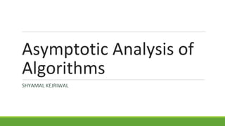
Now that you know the basic operations and data types present in modern
systems, can you analyze the running time and space requirements of the
following C++ code snippets.](https://image.slidesharecdn.com/asymptoticanalysisofalgorithms-141219150952-conversion-gate01/85/Asymptotic-analysis-of-algorithms-pptx-17-320.jpg)


Asymptotic analysis of algorithms.pptx
- 1. Asymptotic Analysis of Algorithms SHYAMAL KEJRIWAL
- 2. Asymptotic Analysis of Algorithms An algorithm is any well-de?ned step-by-step procedure for solving a computational problem. Examples - Problem Input Output Checking if a number is prime A number Yes/No Finding a shortest path between your hostel and your department IITG Map, your hostel name, your dept name Well-defined shortest path Searching an element in an array of numbers An array of numbers Array index
- 3. Asymptotic Analysis of Algorithms An algorithm can be speci?ed in English, as a computer program, or even as a hardware design. There can be many correct algorithms to solve a given problem. Is the correctness of an algorithm enough for its applicability? By the way, how do we know if an algorithm is correct in the first place?
- 4. Asymptotic Analysis of Algorithms The correctness of an algorithm is not enough. We need to analyze the algorithm for efficiency. Efficiency of an algorithm is measured in terms of: ?Execution time (Time complexity) ©C How long does the algorithm take to produce the output? ?The amount of memory required (Space complexity)
- 5. Asymptotic Analysis of Algorithms Let us analyze a few algorithms for space and time requirements. Problem: Given a number n (<=1) as an input, find the count of all numbers between 1 and n (both inclusive) whose factorials are divisible by 5.
- 6. Asymptotic Analysis of Algorithms ALGORITHM BY ALIA 1. Initialize current = 1 and count = 0. 2. Calculate fact = 1*2*ĪŁ*current. 3. Check if fact%5 == 0. If yes, increment count by 1. 4. Increment current by 1. 5. If current == n+1, stop. Else, go to step 2. ALGORITHM BY BOB 1. Initialize current = 1, fact = 1 and count = 0. 2. Calculate fact = fact*current. 3. Check if fact%5 == 0. If yes, increment count by 1. 4. Increment current by 1. 5. If current == n+1, stop. Else, go to step 2.
- 7. Asymptotic Analysis of Algorithms ALGORITHM BY ALIA 1. Initialize current = 1 and count = 0. 2. Calculate fact = 1*2*ĪŁ*current. 3. Check if fact%5 == 0. If yes, increment count by 1. 4. Increment current by 1. 5. If current == n+1, stop. Else, go to step 2. RUNNING TIME ANALYSIS First note that there are few basic operations that are used in this algorithm: 1. Addition (+) 2. Product (*) 3. Modulus (%) 4. Comparison (==) 5. Assignment (=) We assume that each such operation takes constant time Ī░cĪ▒ to execute.
- 8. Asymptotic Analysis of Algorithms ALGORITHM BY ALIA 1. Initialize current = 1 and count = 0. 2. Calculate fact = 1*2*ĪŁ*current. 3. Check if fact%5 == 0. If yes, increment count by 1. 4. Increment current by 1. 5. If current == n+1, stop. Else, go to step 2. RUNNING TIME ANALYSIS Note that different basic operations donĪ»t take same time for execution. Also, the time taken by any single operation also varies from one computation system to other(processor to processor). For simplicity, we assume that each basic operation takes some constant time independent of its nature and computation system on which it is executed. After making the above simplified assumption to analyze running time, we need to calculate the number of times the basic operations are executed in this algorithm. Can you count them?
- 9. Asymptotic Analysis of Algorithms ALGORITHM BY ALIA 1. Initialize current = 1 and count = 0. 2. Calculate fact = 1*2*ĪŁ*current. 3. Check if fact%5 == 0. If yes, increment count by 1. 4. Increment current by 1. 5. If current == n+1, stop. Else, go to step 2. RUNNING TIME ANALYSIS
- 10. Asymptotic Analysis of Algorithms ALGORITHM BY BOB 1. Initialize current = 1, fact = 1 and count = 0. 2. Calculate fact = fact*current. 3. Check if fact%5 == 0. If yes, increment count by 1. 4. Increment current by 1. 5. If current == n+1, stop. Else, go to step 2. RUNNING TIME ANALYSIS Now find the time complexity of the other algorithm for the same problem similarly and appreciate the difference.
- 11. Asymptotic Analysis of Algorithms ALGORITHM BY BOB 1. Initialize current = 1, fact = 1 and count = 0. 2. Calculate fact = fact*current. 3. Check if fact%5 == 0. If yes, increment count by 1. 4. Increment current by 1. 5. If current == n+1, stop. Else, go to step 2. RUNNING TIME ANALYSIS
- 12. Asymptotic Analysis of Algorithms CAN WE DO BETTER Verify if the following algorithm is correct. If n < 5, count = 0. Else, count = n - 4. RUNNING TIME ANALYSIS A constant time algorithm, isnĪ»t it? For such algorithms, we say that the time complexity is ”©(1). Algorithms whose solutions are independent of the size of the problemĪ»s inputs are said to have constant time complexity. Constant time complexity is denoted as ”©(1).
- 13. Asymptotic Analysis of Algorithms The previous examples suggest that we need to know the following two things to calculate running time for an algorithm. 1. What are the basic or constant time operations present in the computation system used to implement the algorithm? 2. How many such basic operations are performed in the algorithm? We count the number of basic operations required in terms of input values or input size.
- 14. Asymptotic Analysis of Algorithms Similarly, to calculate space requirements for an algorithm, we need to answer the following. 1. What are the basic or constant space data types present in the computation system used to implement the algorithm? 2. How many instances of such basic data types are used in the algorithm?
- 15. Asymptotic Analysis of Algorithms Our computer systems generally support following constant time instructions: 1. arithmetic (such as add, subtract, multiply, divide, remainder, ?oor, ceiling) 2. data movement (load, store, copy) 3. control (conditional and unconditional branch, subroutine call and return).
- 16. Asymptotic Analysis of Algorithms The basic data types generally supported in our computer systems are integer and ?oating point (for storing real numbers). Note that characters are also stored as 1 byte integers in our systems. So, if we use few arrays of Ī«nĪ» integers in our algorithm, we can say that the space requirements of the algorithm is proportional to n. Or, the space complexity is ”©(n).
- 17. Asymptotic Analysis of Algorithms int x = 0; for ( int j = 1; j <= n/2; j++ ){ x = x + j; } int n; int *array; cin >> n; array = new int [n]; for ( int j = 0; j < n; j++ ){ array[j] = j + 1; } Now that you know the basic operations and data types present in modern systems, can you analyze the running time and space requirements of the following C++ code snippets.
- 18. Asymptotic Analysis of Algorithms
- 19. Asymptotic Analysis of Algorithms
- 20. Asymptotic Analysis of Algorithms ”© Notation To determine the time complexity of an algorithm: Express the amount of work done as a sum f1(n) + f2(n) + ĪŁ + fk(n) Identify the dominant term: the fi such that fj is ”©(fi) and for k different from j fk(n) < fj(n) (for all sufficiently large n) Then the time complexity is ”©(fi)
- 21. Asymptotic Analysis of Algorithms
- 22. Asymptotic Analysis of Algorithms
- 23. Asymptotic Analysis of Algorithms Let us try analyze a few more C++ codes and express the time and space complexities in ”© notation. With independent nested loops: The number of iterations of the inner loop is independent of the number of iterations of the outer loop int x = 0; for ( int j = 1; j <= n/2; j++ ){ for ( int k = 1; k <= n*n; k++ ){ x = x + j + k; } }
- 24. Asymptotic Analysis of Algorithms Let us try analyze a few more C++ codes and express the time and space complexities in ”© notation. With dependent nested loops: Number of iterations of the inner loop depends on a value from the outer loop int x = 0; for ( int j = 1; j <= n; j++ ){ for ( int k = 1; k <= 3*j; k++ ){ x = x + j; } }
- 25. Asymptotic Analysis of Algorithms ? C++ codes for algorithms discussed and running time analysis ? Linear search vs binary search ? Worst case time complexity