Automatic Dense Semantic Mapping From Visual Street-level Imagery
ŌĆóDownload as PPT, PDFŌĆó
2 likesŌĆó830 views

This talk presented at IROS 2012, Portugal, discusses a method to generate an overhead semantic map, akin to google maps but with associated object class labels. We run experiment on tens of kilometres of data.
![Automatic Dense Semantic Mapping From
Visual Street-level Imagery
Sunando Sengupta[1]
, Paul Sturgess[1]
,
Lubor Ladicky[2]
, Phillip H.S. Torr[1]
[1]
Oxford Brookes University
[2]
Visual geometry group, Oxford University
http://cms.brookes.ac.uk/research/visiongroup/index.php 1](https://image.slidesharecdn.com/iros2012v8-150609074805-lva1-app6892/85/Automatic-Dense-Semantic-Mapping-From-Visual-Street-level-Imagery-1-320.jpg)
![Dense Semantic Map
ŌĆó Street images captured inexpensively from vehicle with
multiple mounted camera[1]
.
3
[1] Yotta. DCL, ŌĆ£Yotta dcl case studies,ŌĆØ Available: http://www.yottadcl.com/surveys/case-
studies/](https://image.slidesharecdn.com/iros2012v8-150609074805-lva1-app6892/85/Automatic-Dense-Semantic-Mapping-From-Visual-Street-level-Imagery-3-320.jpg)


![Semantic Image Segmentation - CRF
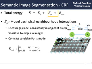
ŌĆó Total energy E = Epix + Epair + Eregion
ŌĆó Epix - Model individual pixelŌĆÖs cost of taking a label.
ŌĆō Computed via the dense boosting approach
ŌĆō Multi feature variant of texton boost[1]
x
Car 0.2
Road 0.3
10[1] L. Ladicky, C. Russell, P. Kohli, and P. H. Torr, ŌĆ£Associative hierarchical crfs for
object class image segmentation,ŌĆØ in ICCV, 2009.](https://image.slidesharecdn.com/iros2012v8-150609074805-lva1-app6892/85/Automatic-Dense-Semantic-Mapping-From-Visual-Street-level-Imagery-10-320.jpg)

![Semantic Image Segmentation
ŌĆó Solved using alpha-expansion algorithm[1]
13
BuildingRoadTreeVegetation FenceSignage
SkyPavement Car Pedestrian Bollard Shop Sign Post
Input Image Road Expansion
[1] Fast Approximate Energy Minimization via Graph Cuts. Yuri Boykov et al. ICCV 99](https://image.slidesharecdn.com/iros2012v8-150609074805-lva1-app6892/85/Automatic-Dense-Semantic-Mapping-From-Visual-Street-level-Imagery-13-320.jpg)
![Semantic Image Segmentation
ŌĆó Solved using alpha-expansion algorithm[1]
14
Input Image Building Expansion
BuildingRoadTreeVegetation FenceSignage
SkyPavement Car Pedestrian Bollard Shop Sign Post
[1] Fast Approximate Energy Minimization via Graph Cuts. Yuri Boykov et al. ICCV 99](https://image.slidesharecdn.com/iros2012v8-150609074805-lva1-app6892/85/Automatic-Dense-Semantic-Mapping-From-Visual-Street-level-Imagery-14-320.jpg)
![Semantic Image Segmentation
ŌĆó Solved using alpha-expansion algorithm[1]
15
Input Image Sky Expansion
BuildingRoadTreeVegetation FenceSignage
SkyPavement Car Pedestrian Bollard Shop Sign Post
[1] Fast Approximate Energy Minimization via Graph Cuts. Yuri Boykov et al. ICCV 99](https://image.slidesharecdn.com/iros2012v8-150609074805-lva1-app6892/85/Automatic-Dense-Semantic-Mapping-From-Visual-Street-level-Imagery-15-320.jpg)
![Semantic Image Segmentation
ŌĆó Solved using alpha-expansion algorithm[1]
16
Input Image Pavement Expansion
BuildingRoadTreeVegetation FenceSignage
SkyPavement Car Pedestrian Bollard Shop Sign Post
[1] Fast Approximate Energy Minimization via Graph Cuts. Yuri Boykov et al. ICCV 99](https://image.slidesharecdn.com/iros2012v8-150609074805-lva1-app6892/85/Automatic-Dense-Semantic-Mapping-From-Visual-Street-level-Imagery-16-320.jpg)
![Semantic Image Segmentation
ŌĆó Solved using alpha-expansion algorithm[1]
17
Input Image Final solution
BuildingRoadTreeVegetation FenceSignage
SkyPavement Car Pedestrian Bollard Shop Sign Post
[1] Fast Approximate Energy Minimization via Graph Cuts. Yuri Boykov et al. ICCV 99](https://image.slidesharecdn.com/iros2012v8-150609074805-lva1-app6892/85/Automatic-Dense-Semantic-Mapping-From-Visual-Street-level-Imagery-17-320.jpg)


![Dataset
ŌĆó Subset of the images captured by the van
ŌĆō 14.8 km of track, 8000 images from each camera.
ŌĆó Pixel-level labelled ground truth images. Dataset
available[1].
ŌĆó 13 object categories ŌĆō
ŌĆó Training - 44 images, testing - 42 images.
[1]http://cms.brookes.ac.uk/research/visiongroup/projects/SemanticMap/index.php
BuildingRoadTreeVegetation FenceSignage
SkyPavement Car Pedestrian Bollard Shop Sign Post
33](https://image.slidesharecdn.com/iros2012v8-150609074805-lva1-app6892/85/Automatic-Dense-Semantic-Mapping-From-Visual-Street-level-Imagery-33-320.jpg)
![SIS Results
ŌĆó Input Images, output of our image level CRF, ground truths.
ŌĆó Used Automatic Labelling environment[1]
[1] The Automatic Labelling Environment, L Ladicky, PHS Torr. Code available
http://cms.brookes.ac.uk/staff/PhilipTorr/ale.htm
BuildingRoadTreeVegetation FenceSignage
SkyPavement Car Pedestrian Bollard Shop Sign Post
34
Input
Semantic
segmentation
Ground Truth](https://image.slidesharecdn.com/iros2012v8-150609074805-lva1-app6892/85/Automatic-Dense-Semantic-Mapping-From-Visual-Street-level-Imagery-34-320.jpg)


![Conclusions
ŌĆó Presented a method to generate
overhead view semantic
mapping.
ŌĆó Experiments on large tracks
(~15km) which can be scaled up
to country wide mapping
ŌĆó Dataset available[1].
[1] http://cms.brookes.ac.uk/research/visiongroup/projects/SemanticMap/index.php
38](https://image.slidesharecdn.com/iros2012v8-150609074805-lva1-app6892/85/Automatic-Dense-Semantic-Mapping-From-Visual-Street-level-Imagery-38-320.jpg)


Automatic Dense Semantic Mapping From Visual Street-level Imagery
- 1. Automatic Dense Semantic Mapping From Visual Street-level Imagery Sunando Sengupta[1] , Paul Sturgess[1] , Lubor Ladicky[2] , Phillip H.S. Torr[1] [1] Oxford Brookes University [2] Visual geometry group, Oxford University http://cms.brookes.ac.uk/research/visiongroup/index.php 1
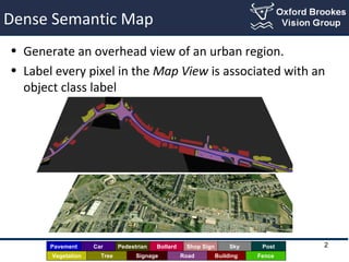
- 2. Dense Semantic Map ŌĆó Generate an overhead view of an urban region. ŌĆó Label every pixel in the Map View is associated with an object class label BuildingRoadTreeVegetation FenceSignage SkyPavement Car Pedestrian Bollard Shop Sign Post 2
- 3. Dense Semantic Map ŌĆó Street images captured inexpensively from vehicle with multiple mounted camera[1] . 3 [1] Yotta. DCL, ŌĆ£Yotta dcl case studies,ŌĆØ Available: http://www.yottadcl.com/surveys/case- studies/
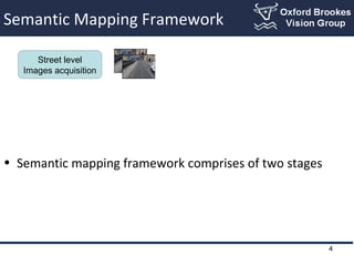
- 4. Semantic Mapping Framework ŌĆó Semantic mapping framework comprises of two stages Street level Images acquisition 4
- 5. Semantic Mapping Framework ŌĆó Semantic mapping framework comprises of two stages ŌĆō Semantic Image Segmentation at street level. Street level Images acquisition Image Segmentation 5
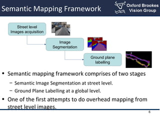
- 6. Semantic Mapping Framework ŌĆó Semantic mapping framework comprises of two stages ŌĆō Semantic Image Segmentation at street level. ŌĆō Ground Plane Labelling at a global level. ŌĆó One of the first attempts to do overhead mapping from street level images. Street level Images acquisition Image Segmentation Ground plane labelling 6
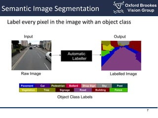
- 7. Semantic Image Segmentation Label every pixel in the image with an object class BuildingRoadTreeVegetation FenceSignage SkyPavement Car Pedestrian Bollard Shop Sign Post Input Output Raw Image Labelled Image Automatic Labeller Object Class Labels 7
- 8. CRFCRF constructionconstruction Semantic Image Segmentation ŌĆó We use Conditional Random Field Framework (CRF) Final SegmentationInput Image 8 ŌĆó Each pixel is a node in a grid graph G = (V,E). ŌĆó Each node is a random variable x taking a label from label set. X
- 9. Semantic Image Segmentation - CRF ŌĆó Total energy ŌĆó Optimal labelling given as 9 ŌłæŌłæŌłæ ŌłłŌłłŌłłŌłł ++= Cc cc NjVi jiij Vi ii i xxxE )(),()()( , xx ŽłŽłŽł Epix Epair Eregion
- 10. Semantic Image Segmentation - CRF ŌĆó Total energy E = Epix + Epair + Eregion ŌĆó Epix - Model individual pixelŌĆÖs cost of taking a label. ŌĆō Computed via the dense boosting approach ŌĆō Multi feature variant of texton boost[1] x Car 0.2 Road 0.3 10[1] L. Ladicky, C. Russell, P. Kohli, and P. H. Torr, ŌĆ£Associative hierarchical crfs for object class image segmentation,ŌĆØ in ICCV, 2009.
- 11. Semantic Image Segmentation - CRF ŌĆó Total energy E = Epix + Epair + Eregion ŌĆó Epair- Model each pixel neighbourhood interactions. ŌĆō Encourages label consistency in adjacent pixels ŌĆō Sensitive to edges in images. ŌĆō Contrast sensitive Potts model xi xj Car Road 0 g(i,j) Car Road 11 Epair
- 12. Semantic Image Segmentation - CRF ŌĆó Total energy E = Epix + Epair + Eregion ŌĆó Eregion - Model behaviour of a group of pixels. ŌĆō Classify a region ŌĆō Encourages all the pixels in a region to take the same label. ŌĆō Group of pixels given by a multiple meanshift segmentations c Car 0.3 Road 0.1 12
- 13. Semantic Image Segmentation ŌĆó Solved using alpha-expansion algorithm[1] 13 BuildingRoadTreeVegetation FenceSignage SkyPavement Car Pedestrian Bollard Shop Sign Post Input Image Road Expansion [1] Fast Approximate Energy Minimization via Graph Cuts. Yuri Boykov et al. ICCV 99
- 14. Semantic Image Segmentation ŌĆó Solved using alpha-expansion algorithm[1] 14 Input Image Building Expansion BuildingRoadTreeVegetation FenceSignage SkyPavement Car Pedestrian Bollard Shop Sign Post [1] Fast Approximate Energy Minimization via Graph Cuts. Yuri Boykov et al. ICCV 99
- 15. Semantic Image Segmentation ŌĆó Solved using alpha-expansion algorithm[1] 15 Input Image Sky Expansion BuildingRoadTreeVegetation FenceSignage SkyPavement Car Pedestrian Bollard Shop Sign Post [1] Fast Approximate Energy Minimization via Graph Cuts. Yuri Boykov et al. ICCV 99
- 16. Semantic Image Segmentation ŌĆó Solved using alpha-expansion algorithm[1] 16 Input Image Pavement Expansion BuildingRoadTreeVegetation FenceSignage SkyPavement Car Pedestrian Bollard Shop Sign Post [1] Fast Approximate Energy Minimization via Graph Cuts. Yuri Boykov et al. ICCV 99
- 17. Semantic Image Segmentation ŌĆó Solved using alpha-expansion algorithm[1] 17 Input Image Final solution BuildingRoadTreeVegetation FenceSignage SkyPavement Car Pedestrian Bollard Shop Sign Post [1] Fast Approximate Energy Minimization via Graph Cuts. Yuri Boykov et al. ICCV 99
- 18. Ground Plane Labelling ŌĆó Combine many labellings from street level imagery. Automatic Labeller Output Labelled Ground PlaneStreet Level labellings Input 18
- 19. Ground Plane CRF ŌĆó A CRF defined over the ground plane. ŌĆó Each ground plane pixel (zi) is a random variable taking a label from the label set. ŌĆó Energy for ground plane crf is Z 19 g pair g pix g EEZE +=)(
- 20. Ground Plane Pixel Cost K X Z ŌĆó We assume a flat world. 20
- 21. Ground Plane Pixel Cost Homography Road Pavement Post/Pole K X Z ŌĆó A ground plane region is estimated. 21
- 22. K X Z Ground Plane Pixel Cost 22 Homography Road Pavement Post/Pole ŌĆó Each point in the image projects to a unique point on the ground plane. ŌĆō Creating a homography
- 23. K X Z Ground Plane Pixel Cost 23 Ground plane Pixel histograms Homography Road Pavement Post/Pole ŌĆó The image labelling is mapped to the ground plane ŌĆō via the homography.
- 24. ŌĆó Labels projected from many views are combined in a histogram. ŌĆó The normalised histogram gives the na├»ve probability of the ground plane pixel taking a label. Ground Plane Pixel Cost 24 K X Z Ground plane Pixel histogramsHomography Road Pavement Post/Pole
- 25. Ground Plane Pixel Cost 25 K X Z Ground plane Pixel histogramsHomography Road Pavement Post/Pole ŌĆó Labels projected from many views are combined in a histogram. ŌĆó The normalised histogram gives the na├»ve probability of the ground plane pixel taking a label.
- 26. Ground Plane labelling ŌĆó Histogram is built for every ground plane pixel giving Eg pix ŌĆó Pairwise cost (Eg pair) added to induce smoothness ŌĆō Contrast sensitive potts model Z
- 27. Ground Plane labelling ŌĆó Final CRF solution obtained using alpha expansion. Void
- 28. Ground Plane labelling Road expansion ŌĆó Final CRF solution obtained using alpha expansion.
- 29. Ground Plane labelling Building expansion ŌĆó Final CRF solution obtained using alpha expansion.
- 30. Ground Plane labelling Pavement expansion ŌĆó Final CRF solution obtained using alpha expansion.
- 31. Ground Plane labelling Car expansion ŌĆó Final CRF solution obtained using alpha expansion.
- 32. Ground Plane Labelling Final Solution ŌĆó Final CRF solution obtained using alpha expansion.
- 33. Dataset ŌĆó Subset of the images captured by the van ŌĆō 14.8 km of track, 8000 images from each camera. ŌĆó Pixel-level labelled ground truth images. Dataset available[1]. ŌĆó 13 object categories ŌĆō ŌĆó Training - 44 images, testing - 42 images. [1]http://cms.brookes.ac.uk/research/visiongroup/projects/SemanticMap/index.php BuildingRoadTreeVegetation FenceSignage SkyPavement Car Pedestrian Bollard Shop Sign Post 33
- 34. SIS Results ŌĆó Input Images, output of our image level CRF, ground truths. ŌĆó Used Automatic Labelling environment[1] [1] The Automatic Labelling Environment, L Ladicky, PHS Torr. Code available http://cms.brookes.ac.uk/staff/PhilipTorr/ale.htm BuildingRoadTreeVegetation FenceSignage SkyPavement Car Pedestrian Bollard Shop Sign Post 34 Input Semantic segmentation Ground Truth
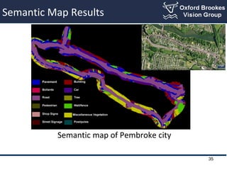
- 35. Semantic Map Results Semantic map of Pembroke city 35
- 36. Ground plane Map Evaluation 36 Street Images Back-projected Map results Ground Truth ŌĆó We back-project the ground plane map into image domain and evaluate the results. ŌĆó Global pixel accuracy of 86%
- 37. Results 37
- 38. Conclusions ŌĆó Presented a method to generate overhead view semantic mapping. ŌĆó Experiments on large tracks (~15km) which can be scaled up to country wide mapping ŌĆó Dataset available[1]. [1] http://cms.brookes.ac.uk/research/visiongroup/projects/SemanticMap/index.php 38
- 39. Future Work 39 Oxford Brookes Vision group Oxford Brookes University http://cms.brookes.ac.uk/research/visiongroup/index.php ŌĆó Perform a 3D street level semantic mapping and reconstruction. ŌĆó Add detailed street level information like signs, information boards etc. Thank you!!!
- 41. Ground Plane Pixel Cost 41 ŌĆó Using single view will create a shadow effect for objects violating flat world assumption and wrong label estimate K X Z Single view Multi-view Homography Road Pavement Post/Pole
Editor's Notes
- #3: In this work where we create a Dense semantic map of an urban region. By Dense semantic map we mean an overhead birdŌĆÖs eye view of a region associated with object labels This image shows a street image (below ) and the associated labelled map on the top. Adding semantic information helps in making an autonomous vehicle help to understand its surroundings. With dense mapping a better boundary estimate can be achieved which helps in navigation for autonomous vehicles in structured environments.
- #4: For this purpose we use street level images captured from cameras mounted on a vehicle. Street level images can be taken in an relatively inexpensive manner, e.g. using cameras in vehicle. They are often generally more detailed and can be captured in high frequency. They have a wealth of semantic information that can be exploited effectively to our purpose. In our experiments the images are captured by a highway maping company called yotta. The have taken images across hundreds of kmŌĆÖs across UK which consists of urban, semi urban and highway images.
- #5: Our frame work of semantic mapping consists of broadly two parts. The semantic mapping framework comprises of two main stages. Once the street level images are acquired, the semantic image segmentation is performed on them individually. These results at local level are aggregated and fed into a global ground plane labelling system which outputs our dense semantic map.
- #6: Our frame work of semantic mapping consists of broadly two parts. The semantic mapping framework comprises of two main stages. Once the street level images are acquired, the semantic image segmentation is performed on them individually. These results at local level are aggregated and fed into a global ground plane labelling system which outputs our dense semantic map.
- #7: Our frame work of semantic mapping consists of broadly two parts. The semantic mapping framework comprises of two main stages. Once the street level images are acquired, the semantic image segmentation is performed on them individually. These results at local level are aggregated and fed into a global ground plane labelling system which outputs our dense semantic map.
- #8: In this section we talk about the image segmentation/labelling problem. The image segmentation problem is to label every image pixels in the image into a particular class label such as car, road , building etc. Labelling is a hard problem, exponential number of possibility (millions of pixels, 10-100ŌĆÖs of labels). We would like to have a system where we give an input street image to an automatic labeller which will give us a semantically labelled image., like in this example telling where is road/car/pavement/building etc.
- #9: We use Conditional Random field (CRF). This has achieved state of the art results in classification of road scene data in recent years. In this framework,. The image is described as a grid graph. All the pixels in the image are the vertices of the graph. each pixel is modelled as a variable which takes a value from the label set which we need to find out.
- #10: We define an cost on the graph, whose components are given by the nodes which is called as Epix, , edges calles as E pairs and the region (E regions). The final labelling is given by x that minimises this energy.
- #11: We now define each of the energy component in details. Epix models the individual pixels cost of taking a label. Generally this is the classifier cost. In our case it is computed via the boosting approach. This is shown in the example, the green node has the cost of taking the label car.2 and road 0.1. similarly all the cost of other nodes are also computed.
- #12: The next cost item is the pairwise cost which models the pixel neighbourhood region. This kind of cost will try to enforce the consistency in label among adjacent pixels. Thus it is Sensitive to edges and preserves boundaries in images. Here in this example you can see the cost of two pixels taking the same label car is zero but non zero otherwise.
- #13: The final cost terms models the behaviour of the group of the pixels defining a region. Here the region is found by unsupervised segmentetiontion technique like manshift, and encourages the entire region to be classified into a same class label. In this example the entire clique will take a cost for an object label.
- #14: Solved in a graph cut approach. This is the alpha expansion inference. In each step, one of the label is expanded (which results in lowering the energy) and the entire process is iterated for a number of times. Here in this example first we show the expansion step for road, then building, then sky. Finally we achieve at the final solution when there is no reduction in energy value.
- #16: Solved in a graph cut approach. This is the alpha expansion inference. In each step, one of the label is expanded (which results in lowering the energy) and the entire process is iterated for a number of times. Here in this example first we show the expansion step for road, then building, then sky. Finally we achieve at the final solution when there is no reduction in energy value.
- #17: Solved in a graph cut approach. This is the alpha expansion inference. In each step, one of the label is expanded (which results in lowering the energy) and the entire process is iterated for a number of times. Here in this example first we show the expansion step for road, then building, then sky. Finally we achieve at the final solution when there is no reduction in energy value.
- #18: Solved in a graph cut approach. This is the alpha expansion inference. In each step, one of the label is expanded (which results in lowering the energy) and the entire process is iterated for a number of times. Here in this example first we show the expansion step for road, then building, then sky. Finally we achieve at the final solution when there is no reduction in energy value.
- #19: In this stage all the semantically segmented street images are aggregated and fed into an labeller which will output the ground plane map.
- #20: A graph is defined over the ground plane , and each pixel of the ground plane is a vertex/node in the graph, with adjacent vertices connected. For each ground plane pixel a voting scheme determines the cost of the label it takes. The pairwise connections are added to get smoothes in the output solution.
- #21: Firstly for aggregation of results to determine the per-pixel classifier cost in the ground plane , we assume a flat world. We define a ground plane patch given the camera viewing direction and project it on to the camera. This gives us a relationship between the image and the ground plane.
- #22: Firstly for aggregation of results to determine the per-pixel classifier cost in the ground plane , we assume a flat world. We define a ground plane patch given the camera viewing direction and project it on to the camera. This gives us a relationship between the image and the ground plane.
- #23: Firstly for aggregation of results to determine the per-pixel classifier cost in the ground plane , we assume a flat world. We define a ground plane patch given the camera viewing direction and project it on to the camera. This gives us a relationship between the image and the ground plane.
- #24: A histogram of label prediction is build for ground plane pixel by aggregating in a voting manner
- #25: Multiple view is added accross time and cameras
- #34: Our dataset consist of the subset of all the images taken by the Yotta dcl. We work on images of 14.8 km road track. The images are from Pembroke city UK. We have labelled the images and made the dataset available. We have 13 object categories. Split the training /testing as 44/42 images. The training images are taken in a small but representative subset of the data.
- #35: First row shows the street images, and the object labelling in the second row. The last row denotes the corresponding ground truth.
- #36: This example shows the semantic map result. In the top-right we can see the track of the vehicle taking images.
- #37: As the semantic labelling of a ground plane map is expensive, we use a back-projection method to evaluate the map. We project the ground plane map results into the image domain and evaluate in the image domain Labelling of ground plane from google maps is expensive and
- #38: This video shows our output. Firs we see the images taken by the car, as the car moves around pembroke city UK. The street level images are semantically segmented in the crf framework. These information are aggregated to build the map. The map is continuously updated as more and more information is added from the street level images. We can see the vehicle turns which is reflected in the map. This is a closeup view of the map, with pavement and cars being shown in the map and the images. Cars in the images captured in the image and shown in the map. This is another close up view where the pavement is flanked by the road and car-park. This is captured in the overhead generated map.
- #39: Finally to conclude, we have presented a method of performing a dense sematic mapping . We showed experiments on large track of data, and we make this dataset available. We hope to make it real time in future with fast binary features and fast maen field based inference for labelling. Thank you.
- #40: Thank you
- #43: Multiple view is added accross time and cameras