Backpropagation - A peek into the Mathematics of optimization.pdf
ŌĆó
0 likesŌĆó27 views

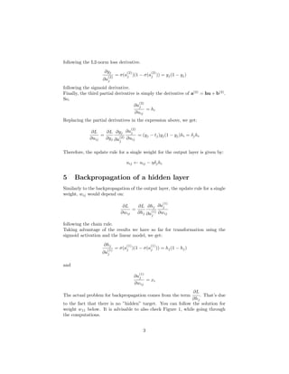
This document introduces backpropagation, which is the core optimization process in deep neural networks. It summarizes backpropagation for both the output layer and hidden layers. For the output layer, the update rule for a single weight is given by uij ŌåÉ uij - ╬Ę╬┤jhi, where ╬┤j = (yj - tj)yj(1-yj). For the hidden layer, the update rule is more complex, with ŌłéL/Ōłéwij = ╬Żk(yk - tk)yk(1-yk)ujkhj(1-hj)xi. Finally, it provides a generalized backpropagation formula that combines these rules for both layers as ŌłéL

![ŌłéL
Ōłéh1
=
ŌłéL
Ōłéy1
Ōłéy1
Ōłéa
(2)
1
Ōłéa
(2)
1
Ōłéh1
+
ŌłéL
Ōłéy2
Ōłéy2
Ōłéa
(2)
2
Ōłéa
(2)
2
Ōłéh1
=
= (y1 ŌłÆ t1)y1(1 ŌłÆ y1)u11 + (y2 ŌłÆ t2)y2(1 ŌłÆ y2)u12
From here, we can calculate
ŌłéL
Ōłéw11
, which was what we wanted. The final ex-
pression is:
ŌłéL
Ōłéw11
= [(y1 ŌłÆ t1)y1(1 ŌłÆ y1)u11 + (y2 ŌłÆ t2)y2(1 ŌłÆ y2)u12] h1(1 ŌłÆ h1)x1
The generalized form of this equation is:
ŌłéL
Ōłéwij
=
X
k
(yk ŌłÆ tk)yk(1 ŌłÆ yk)ujkhj(1 ŌłÆ hj)xi
6 Backpropagation generalization
Using the results for backpropagation for the output layer and the hidden layer,
we can put them together in one formula, summarizing backpropagation, in the
presence of L2-norm loss and sigmoid activations.
ŌłéL
Ōłéwij
= ╬┤jxi
where for a hidden layer
╬┤j =
X
k
╬┤kwjkyj(1 ŌłÆ yj)
Kudos to those of you who got to the end.
Thanks for reading.
4](https://image.slidesharecdn.com/backpropagation-apeekintothemathematicsofoptimization-221207092652-448d72c0/85/Backpropagation-A-peek-into-the-Mathematics-of-optimization-pdf-4-320.jpg)
Backpropagation - A peek into the Mathematics of optimization.pdf
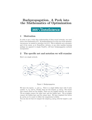
- 1. Backpropagation. A Peek into the Mathematics of Optimization 1 Motivation In order to get a truly deep understanding of deep neural networks, one must look at the mathematics of it. As backpropagation is at the core of the optimiza- tion process, we wanted to introduce you to it. This is definitely not a necessary part of the course, as in TensorFlow, sk-learn, or any other machine learning package (as opposed to simply NumPy), will have backpropagation methods incorporated. 2 The specific net and notation we will examine HereŌĆÖs our simple network: Figure 1: Backpropagation We have two inputs: x1 and x2. There is a single hidden layer with 3 units (nodes): h1, h2, and h3. Finally, there are two outputs: y1 and y2. The arrows that connect them are the weights. There are two weights matrices: w, and u. The w weights connect the input layer and the hidden layer. The u weights connect the hidden layer and the output layer. We have employed the letters w, and u, so it is easier to follow the computation to follow. You can also see that we compare the outputs y1 and y2 with the targets t1 and t2. 1
- 2. There is one last letter we need to introduce before we can get to the compu- tations. Let a be the linear combination prior to activation. Thus, we have: a(1) = xw + b(1) and a(2) = hu + b(2) . Since we cannot exhaust all activation functions and all loss functions, we will focus on two of the most common. A sigmoid activation and an L2-norm loss. With this new information and the new notation, the output y is equal to the ac- tivated linear combination. Therefore, for the output layer, we have y = Žā(a(2) ), while for the hidden layer: h = Žā(a(1) ). We will examine backpropagation for the output layer and the hidden layer separately, as the methodologies differ. 3 Useful formulas I would like to remind you that: L2-norm loss: L = 1 2 X i (yi ŌłÆ ti)2 The sigmoid function is: Žā(x) = 1 1 + eŌłÆx and its derivative is: Žā0 (x) = Žā(x)(1 ŌłÆ Žā(x)) 4 Backpropagation for the output layer In order to obtain the update rule: u ŌåÉ u ŌłÆ ╬ĘŌłćuL(u) we must calculate ŌłćuL(u) LetŌĆÖs take a single weight uij. The partial derivative of the loss w.r.t. uij equals: ŌłéL Ōłéuij = ŌłéL Ōłéyj Ōłéyj Ōłéa (2) j Ōłéa (2) j Ōłéuij where i corresponds to the previous layer (input layer for this transformation) and j corresponds to the next layer (output layer of the transformation). The partial derivatives were computed simply following the chain rule. ŌłéL Ōłéyj = (yj ŌłÆ tj) 2
- 3. following the L2-norm loss derivative. Ōłéyj Ōłéa (2) j = Žā(a (2) j )(1 ŌłÆ Žā(a (2) j )) = yj(1 ŌłÆ yj) following the sigmoid derivative. Finally, the third partial derivative is simply the derivative of a(2) = hu + b(2) . So, Ōłéa (2) j Ōłéuij = hi Replacing the partial derivatives in the expression above, we get: ŌłéL Ōłéuij = ŌłéL Ōłéyj Ōłéyj Ōłéa (2) j Ōłéa (2) j Ōłéuij = (yj ŌłÆ tj)yj(1 ŌłÆ yj)hi = ╬┤jhi Therefore, the update rule for a single weight for the output layer is given by: uij ŌåÉ uij ŌłÆ ╬Ę╬┤jhi 5 Backpropagation of a hidden layer Similarly to the backpropagation of the output layer, the update rule for a single weight, wij would depend on: ŌłéL Ōłéwij = ŌłéL Ōłéhj Ōłéhj Ōłéa (1) j Ōłéa (1) j Ōłéwij following the chain rule. Taking advantage of the results we have so far for transformation using the sigmoid activation and the linear model, we get: Ōłéhj Ōłéa (1) j = Žā(a (1) j )(1 ŌłÆ Žā(a (1) j )) = hj(1 ŌłÆ hj) and Ōłéa (1) j Ōłéwij = xi The actual problem for backpropagation comes from the term ŌłéL Ōłéhj . ThatŌĆÖs due to the fact that there is no ŌĆØhiddenŌĆØ target. You can follow the solution for weight w11 below. It is advisable to also check Figure 1, while going through the computations. 3
- 4. ŌłéL Ōłéh1 = ŌłéL Ōłéy1 Ōłéy1 Ōłéa (2) 1 Ōłéa (2) 1 Ōłéh1 + ŌłéL Ōłéy2 Ōłéy2 Ōłéa (2) 2 Ōłéa (2) 2 Ōłéh1 = = (y1 ŌłÆ t1)y1(1 ŌłÆ y1)u11 + (y2 ŌłÆ t2)y2(1 ŌłÆ y2)u12 From here, we can calculate ŌłéL Ōłéw11 , which was what we wanted. The final ex- pression is: ŌłéL Ōłéw11 = [(y1 ŌłÆ t1)y1(1 ŌłÆ y1)u11 + (y2 ŌłÆ t2)y2(1 ŌłÆ y2)u12] h1(1 ŌłÆ h1)x1 The generalized form of this equation is: ŌłéL Ōłéwij = X k (yk ŌłÆ tk)yk(1 ŌłÆ yk)ujkhj(1 ŌłÆ hj)xi 6 Backpropagation generalization Using the results for backpropagation for the output layer and the hidden layer, we can put them together in one formula, summarizing backpropagation, in the presence of L2-norm loss and sigmoid activations. ŌłéL Ōłéwij = ╬┤jxi where for a hidden layer ╬┤j = X k ╬┤kwjkyj(1 ŌłÆ yj) Kudos to those of you who got to the end. Thanks for reading. 4