


![ContŌĆ”
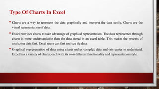
4. CONCATENATE
ŌĆó This function merges or joins several text strings into one text string.
ŌĆó =CONCATENATE(cell, " ", cell)
5. LEN
ŌĆó The function LEN() returns the total number of characters in a string. So, it will count the
overall characters, including spaces and special characters.
ŌĆó =LEN(cell)
6. SUBSTITUTE
ŌĆó The SUBSTITUTE() function replaces the existing text with a new text in a text string.
ŌĆó The syntax is ŌĆ£=SUBSTITUTE(text, old_text, new_text, [instance_num])ŌĆØ.
ŌĆó =SUBSITUTE(text,ŌĆØold-textŌĆØ,ŌĆØnew-textŌĆØ,num).
ŌĆó Here, [instance_num] refers to the index position of the present texts more than once.](https://image.slidesharecdn.com/basiccomputerskill-p4excel-220719152208-15147718/85/Basic-Computer-skill-P4-Excel-pptx-42-320.jpg)
![ContŌĆ”
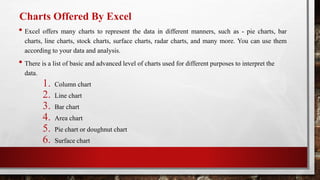
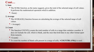
10. VLOOKUP
ŌĆó VLOOKUP() function stands for the vertical lookup that is responsible for looking for a
particular value in the leftmost column of a table. It then returns a value in the same row from
a column you specify.
ŌĆó Below are the arguments for the VLOOKUP function:
ŌĆó Lookup_value - this is the value that you have to look for in the first column of a table.
ŌĆó Table - this indicates the table from which the value is retrieved.
ŌĆó Col_index - the column in the table from the value is to be retrieved.
ŌĆó Range_lookup - [optional] true = approximate match (default). FALSE = exact match.
ŌĆó We will use the below table to learn how the VLOOKUP function works.](https://image.slidesharecdn.com/basiccomputerskill-p4excel-220719152208-15147718/85/Basic-Computer-skill-P4-Excel-pptx-45-320.jpg)
![ContŌĆ”
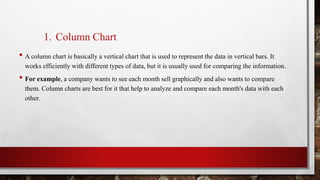
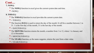
11. HLOOKUP()
ŌĆó HLOOKUP() or horizontal lookup. The function HLOOKUP looks for a value in the top row
of a table or array of benefits. It gives the value in the same column from a row you specify.
ŌĆó Below are the arguments for the HLOOKUP() function:
ŌĆó Lookup_value - this indicates the value to lookup.
ŌĆó Table - this is the table from which you have to retrieve data.
ŌĆó Row_index - this is the row number from which to retrieve data.
ŌĆó Range_lookup - [optional] this is a Boolean to indicate an exact match or approximate match.
The default value is TRUE, meaning an approximate match.](https://image.slidesharecdn.com/basiccomputerskill-p4excel-220719152208-15147718/85/Basic-Computer-skill-P4-Excel-pptx-46-320.jpg)
![ContŌĆ”
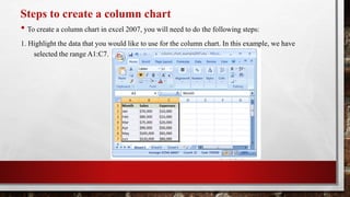
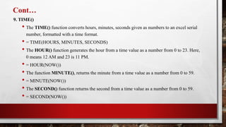
12. Sort()
ŌĆó The excel SORT function sorts the contents of a range or array in ascending or descending
order. Values can be sorted by one or more columns. SORT returns a dynamic array of
results.
ŌĆó =Sort (array, [sort_index], [sort_order], [by_col])
ŌĆó Array - range or array to sort.
ŌĆó Sort_index - [optional] column index to use for sorting. Default is 1.
ŌĆó Sort_order - [optional] 1 = ascending, -1 = descending. Default is ascending order.
ŌĆó By_col - [optional] true = sort by column. FALSE = sort by row. Default is FALSE.
ŌĆó =SORT(B5:C14,1,-1) // sort by scores in descending order
ŌĆó =SORT(B5:C14,1,1) // sort by score in ascending order](https://image.slidesharecdn.com/basiccomputerskill-p4excel-220719152208-15147718/85/Basic-Computer-skill-P4-Excel-pptx-47-320.jpg)

Basic Computer skill-P4 Excel.pptx
- 1. BASIC COMPUTER SKILL PART FOUR Working with office package software
- 2. Microsoft Office Excel ŌĆó Microsoft excel is a spreadsheet program included in the Microsoft office suite of applications. Spreadsheets will provide you with the values arranged in rows and columns that can be changed mathematically using both basic and complex arithmetic operations. ŌĆó Microsoft excel was first released for Macintosh systems in the year 1985, followed by the first windows version in 1987. ŌĆó Can record data in the form of tables. It is easy to analyze data in an excel spreadsheet.
- 3. ContŌĆ” ŌĆó Open excel by using the start menu type Microsoft office excel or by double-clicking the desktop icon for excel ŌĆó Open Microsoft Excel 2007. The Microsoft Excel window appears and your screen looks similar to the one shown here.
- 4. ContŌĆ” Office Button ŌĆó In the upper-left corner of the Excel 2007 window is the Office button. When you click the button, a menu appears. You can use the menu to create a new file, open an existing file, save a file, and perform many other tasks. The Quick Access Toolbar The Quick Access Toolbar is located all the way to the left on the Title Bar. It contains frequently used commands and can be customized using the drop-down menu. Click the Customize Quick Access Toolbar button, check New on the menu. Notice how a new button has appeared.
- 5. ContŌĆ” ŌĆó Click the customize quick access toolbar button again and select show below the ribbon. This repositions the toolbar to be below the ribbon. ŌĆó Note that when the toolbar is below the ribbon, its customize button is very difficult to see, due to its white color. ŌĆó Move the Quick Access Toolbar back above the ribbon by clicking the customize button and selecting Show Above the Ribbon.
- 6. ContŌĆ” Title Bar 1. The title bar section which has window controls at the right end, as in other Microsoft office programs. 2. That a blank workbook opens with a default file name of book1. Ribbon ŌĆó The ribbon contains all of the tools that you use to interact with your Microsoft excel file. It is located at the top of the window. All of the programs in the Microsoft office suite have one. ŌĆó The ribbon has a number of tabs, each of which contains buttons, which are organized into groups.
- 7. ContŌĆ” Workspace ŌĆó Name box: displays the currently selected cell. ŌĆó Formula bar: displays the number, text, or formula that is in the currently selected cell, and allows you to edit it. It behaves just like a text box. ŌĆó Selected cell: the selected cell has a dark border around it. ŌĆó Column: columns run vertically (top to bottom). ŌĆó Column Label: identifies each column with a letter. Clicking on a column label selects the entire column.
- 8. ContŌĆ” ŌĆó Row: rows run horizontally (left to right). ŌĆó Row Label: identifies each row with a number. Clicking on a row label selects the entire row. ŌĆó Cell: the intersection of a row and column. ŌĆó Worksheets: the worksheets contained in the workbook are displayed at the bottom-left of the screen. Click on a worksheet to view it. ŌĆó Scroll bars: used to view other parts of a worksheet when the entire worksheet cannot fit on the screen. ŌĆó View tools: Status Bar The status bar is located below the document window area.
- 9. ContŌĆ” Current Information ŌĆó The left end gives current information about the spreadsheet. Views ŌĆó At the right end are shortcuts to the different views that are available. Each view displays the spreadsheet in a different way, allowing you to carry out various tasks more efficiently. Normal ŌĆó This is the view we will be working in throughout this course. It simply displays the grid of cells that make up your spreadsheet. Page Layout ŌĆó Shows what your spreadsheet will look like when printed on paper. Page Break ŌĆó Preview Allows you to add page breaks to your spreadsheet so you can better control what parts of the spreadsheet are printed on each page.
- 10. ContŌĆ” How to perform arithmetic operations in excel ŌĆó we are going to perform basic arithmetic operations: Addition, subtraction, division and multiplication. The following table shows the data that we will work with and the results that we should expect. S/n Arithmetic operator First number Second number Result 1 Addition (+) 13 3 2 Subtraction (-) 21 9 3 Division (/) 33 12 4 Multiplication (*) 7 3
- 11. ContŌĆ” Step 1) create an excel sheet and enter the data ŌĆó Create a folder on your computer in my documents folder and name it first practice ŌĆó Enter the data in your worksheet as shown in the above. ŌĆó We will now perform the calculations using the respective arithmetic operators. When performing calculations in excel, you should always start with the equal (=) sign Step 2) make column names bold ŌĆó Highlight the cells that have the column names by dragging them. ŌĆó Click on the bold button represented by B command
- 12. ContŌĆ” ŌĆó Step 3) enclose data in boxes ŌĆó Highlight all the columns and rows with data ŌĆó On the font ribbon bar, click on borders command as shown below.
- 13. ContŌĆ” You will get the following drop down menu
- 14. ContŌĆ” ŌĆó Select the option ŌĆ£all bordersŌĆØ. ŌĆó Your data should now look as follows
- 15. Type Of Charts In Excel ŌĆó Charts are a way to represent the data graphically and interpret the data easily. Charts are the visual representation of data. ŌĆó Excel provides charts to take advantage of graphical representation. The data represented through charts is more understandable than the data stored in an excel table. This makes the process of analyzing data fast. Excel users can fast analyze the data. ŌĆó Graphical representation of data using charts makes complex data analysis easier to understand. Excel has a variety of charts, each with its own different functionality and representation style.
- 16. Charts Offered By Excel ŌĆó Excel offers many charts to represent the data in different manners, such as - pie charts, bar charts, line charts, stock charts, surface charts, radar charts, and many more. You can use them according to your data and analysis. ŌĆó There is a list of basic and advanced level of charts used for different purposes to interpret the data. 1. Column chart 2. Line chart 3. Bar chart 4. Area chart 5. Pie chart or doughnut chart 6. Surface chart
- 17. 1. Column Chart ŌĆó A column chart is basically a vertical chart that is used to represent the data in vertical bars. It works efficiently with different types of data, but it is usually used for comparing the information. ŌĆó For example, a company wants to see each month sell graphically and also wants to compare them. Column charts are best for it that help to analyze and compare each month's data with each other.
- 18. Steps to create a column chart ŌĆó To create a column chart in excel 2007, you will need to do the following steps: 1. Highlight the data that you would like to use for the column chart. In this example, we have selected the range A1:C7.
- 19. ContŌĆ” 2. Select the insert tab in the toolbar at the top of the screen. Click on the column button in the charts group and then select a chart from the drop down menu. In this example, we have selected the first column chart (called clustered column) in the 2-D column section.
- 20. ContŌĆ” 3. Now you will see the column chart appear in your spreadsheet with rectangular bars to represent both the sales and the expense numbers. The sales values are displayed as blue vertical bars and the expenses are displayed as red vertical bars. You can see the axis values on the left side of the graph for these vertical bars.
- 21. ContŌĆ” ŌĆó Finally, let's add a title for the column chart. By default, your chart will be created without a title in excel 2007. ŌĆó To add a title, select the layout tab under chart tools in the toolbar at the top of the screen (chart tools will only appear when you have the chart selected). Click on the chart title button in the labels group and then select "above chart" from the drop down menu.
- 22. ContŌĆ” ŌĆó Now you should see a title appear at the top of the chart area. Click on the title and it will become editable. Enter the text that you would like to see as the title. In this tutorial, we have entered "sales and expenses" as the title for the column chart.
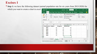
- 23. Excises 1 ŌĆó Step 1: we have the following dataset (animal population rate for six years from 2015-2020) for which you want to create a chart in excel.
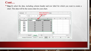
- 24. ContŌĆ” ŌĆó Step 2: select the data, including column header and row label for which you want to create a chart. This data will be the source data for your chart.
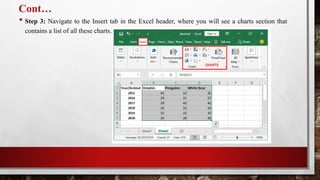
- 25. ContŌĆ” ŌĆó Step 3: Navigate to the Insert tab in the Excel header, where you will see a charts section that contains a list of all these charts.
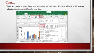
- 26. ContŌĆ” ŌĆó Step 4: choose a chart from here according to your data. We have chosen a 3D column chart containing vertical bars for your data.
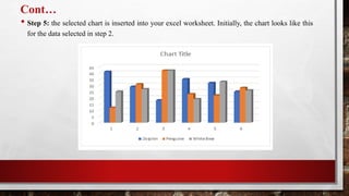
- 27. ContŌĆ” ŌĆó Step 5: the selected chart is inserted into your excel worksheet. Initially, the chart looks like this for the data selected in step 2.
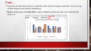
- 28. ContŌĆ” ŌĆó Currently, this chart does not have a valid title, clear values for analysis, and more. You can set up all these things in your chart by modifying it. ŌĆó Step 6: double-tap on the chart title to make it editable and then provide a new valid title that suites to it.
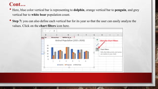
- 29. ContŌĆ” ŌĆó Here, blue color vertical bar is representing to dolphin, orange vertical bar to penguin, and grey vertical bar to white bear population count. ŌĆó Step 7: you can also define each vertical bar for its year so that the user can easily analyze the values. Click on the chart filters icon here.
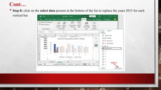
- 30. ContŌĆ” ŌĆó Step 8: click on the select data present at the bottom of the list to replace the years 2015 for each vertical bar.
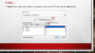
- 31. ContŌĆ” ŌĆó Step 9: here, select the number 1 to replace it with year 2015 and click the edit button.
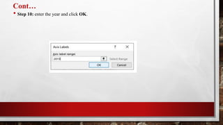
- 32. ContŌĆ” ŌĆó Step 10: enter the year and click OK.
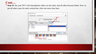
- 33. ContŌĆ” ŌĆó Step 11: the year 2015 will immediately reflect on the chart, and all other become blank. Now, to put all other years for each vertical bar, click one more time here.
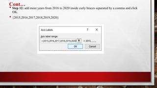
- 34. ContŌĆ” ŌĆó Step 12: add more years from 2016 to 2020 inside curly braces separated by a comma and click OK. ŌĆó {2015,2016,2017,2018,2019,2020}
- 35. ContŌĆ” ŌĆó Step 13: all values are now added. So, click OK.
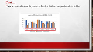
- 36. ContŌĆ” ŌĆó Step 14: see the charts that the years are reflected on the chart correspond to each vertical bar.
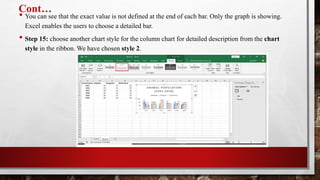
- 37. ContŌĆ” ŌĆó You can see that the exact value is not defined at the end of each bar. Only the graph is showing. Excel enables the users to choose a detailed bar. ŌĆó Step 15: choose another chart style for the column chart for detailed description from the chart style in the ribbon. We have chosen style 2.
- 38. ContŌĆ” ŌĆó Step 16: you can now see the exact value is also showing for each bar in this chart.
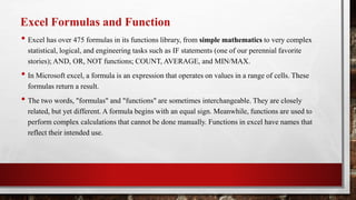
- 39. Excel Formulas and Function ŌĆó Excel has over 475 formulas in its functions library, from simple mathematics to very complex statistical, logical, and engineering tasks such as IF statements (one of our perennial favorite stories); AND, OR, NOT functions; COUNT, AVERAGE, and MIN/MAX. ŌĆó In Microsoft excel, a formula is an expression that operates on values in a range of cells. These formulas return a result. ŌĆó The two words, "formulas" and "functions" are sometimes interchangeable. They are closely related, but yet different. A formula begins with an equal sign. Meanwhile, functions are used to perform complex calculations that cannot be done manually. Functions in excel have names that reflect their intended use.
- 40. ContŌĆ” ŌĆó The example below shows how we have used the multiplication formula manually with the ŌĆś*ŌĆÖ operator. ŌĆó This example below shows how we have used the function - ŌĆśPRODUCTŌĆÖ to perform multiplication. As you can see, we didnŌĆÖt use the mathematical operator here.
- 41. ContŌĆ” 1. Sum ŌĆó The SUM() function, as the name suggests, gives the total of the selected range of cell values. It performs the mathematical operation which is addition. ŌĆó =Sum() 2. Average ŌĆó The AVERAGE() function focuses on calculating the average of the selected range of cell values. ŌĆó = Average() 3. Count ŌĆó The function COUNT() counts the total number of cells in a range that contains a number. It does not include the cell, which is blank, and the ones that hold data in any other format apart from numeric. ŌĆó =Count() ŌĆó To count the number of blank cells present in a range of cells, =COUNTBLANK() is used.
- 42. ContŌĆ” 4. CONCATENATE ŌĆó This function merges or joins several text strings into one text string. ŌĆó =CONCATENATE(cell, " ", cell) 5. LEN ŌĆó The function LEN() returns the total number of characters in a string. So, it will count the overall characters, including spaces and special characters. ŌĆó =LEN(cell) 6. SUBSTITUTE ŌĆó The SUBSTITUTE() function replaces the existing text with a new text in a text string. ŌĆó The syntax is ŌĆ£=SUBSTITUTE(text, old_text, new_text, [instance_num])ŌĆØ. ŌĆó =SUBSITUTE(text,ŌĆØold-textŌĆØ,ŌĆØnew-textŌĆØ,num). ŌĆó Here, [instance_num] refers to the index position of the present texts more than once.
- 43. ContŌĆ” 7. NOW() ŌĆó The NOW() function in excel gives the current system date and time. ŌĆó =NOW() 8. TODAY() ŌĆó The TODAY() function in excel provides the current system date. ŌĆó = TODAY() ŌĆó The function DAY() is used to return the day of the month. It will be a number between 1 to 31. 1 is the first day of the month, 31 is the last day of the month. ŌĆó = DAY(TODAY()) ŌĆó The MONTH() function returns the month, a number from 1 to 12, where 1 is January and 12 is December. ŌĆó = MONTH(TODAY()) ŌĆó The YEAR() function, as the name suggests, returns the year from a date value. ŌĆó = YEAR(TODAY())
- 44. ContŌĆ” 9. TIME() ŌĆó The TIME() function converts hours, minutes, seconds given as numbers to an excel serial number, formatted with a time format. ŌĆó = TIME(HOURS, MINUTES, SECONDS) ŌĆó The HOUR() function generates the hour from a time value as a number from 0 to 23. Here, 0 means 12 AM and 23 is 11 PM. ŌĆó = HOUR(NOW()) ŌĆó The function MINUTE(), returns the minute from a time value as a number from 0 to 59. ŌĆó = MINUTE(NOW()) ŌĆó The SECOND() function returns the second from a time value as a number from 0 to 59. ŌĆó = SECOND(NOW())
- 45. ContŌĆ” 10. VLOOKUP ŌĆó VLOOKUP() function stands for the vertical lookup that is responsible for looking for a particular value in the leftmost column of a table. It then returns a value in the same row from a column you specify. ŌĆó Below are the arguments for the VLOOKUP function: ŌĆó Lookup_value - this is the value that you have to look for in the first column of a table. ŌĆó Table - this indicates the table from which the value is retrieved. ŌĆó Col_index - the column in the table from the value is to be retrieved. ŌĆó Range_lookup - [optional] true = approximate match (default). FALSE = exact match. ŌĆó We will use the below table to learn how the VLOOKUP function works.
- 46. ContŌĆ” 11. HLOOKUP() ŌĆó HLOOKUP() or horizontal lookup. The function HLOOKUP looks for a value in the top row of a table or array of benefits. It gives the value in the same column from a row you specify. ŌĆó Below are the arguments for the HLOOKUP() function: ŌĆó Lookup_value - this indicates the value to lookup. ŌĆó Table - this is the table from which you have to retrieve data. ŌĆó Row_index - this is the row number from which to retrieve data. ŌĆó Range_lookup - [optional] this is a Boolean to indicate an exact match or approximate match. The default value is TRUE, meaning an approximate match.
- 47. ContŌĆ” 12. Sort() ŌĆó The excel SORT function sorts the contents of a range or array in ascending or descending order. Values can be sorted by one or more columns. SORT returns a dynamic array of results. ŌĆó =Sort (array, [sort_index], [sort_order], [by_col]) ŌĆó Array - range or array to sort. ŌĆó Sort_index - [optional] column index to use for sorting. Default is 1. ŌĆó Sort_order - [optional] 1 = ascending, -1 = descending. Default is ascending order. ŌĆó By_col - [optional] true = sort by column. FALSE = sort by row. Default is FALSE. ŌĆó =SORT(B5:C14,1,-1) // sort by scores in descending order ŌĆó =SORT(B5:C14,1,1) // sort by score in ascending order
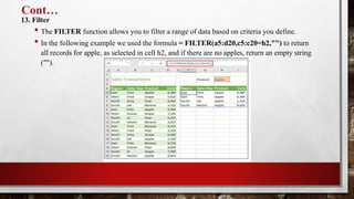
- 48. ContŌĆ” 13. Filter ŌĆó The FILTER function allows you to filter a range of data based on criteria you define. ŌĆó In the following example we used the formula = FILTER(a5:d20,c5:c20=h2,"") to return all records for apple, as selected in cell h2, and if there are no apples, return an empty string ("").
- 49. ░š▒ß┤Ī▒Ę░Ł│¦!ŌĆ”