Bayesian Decision Theory details ML.pptx
- 2. Bayesian Decision Theory 1. Introduction ©C Bayesian Decision Theory ? Pure statistics, probabilities known, optimal decision 2. Bayesian Decision Theory©CContinuous Features 3. Minimum-Error-Rate Classification 4. Classifiers, Discriminant Functions, Decision Surfaces 5. The Normal Density 6. Discriminant Functions for the Normal Density
- 3. 2 1. Introduction ? The sea bass/salmon example ? State of nature, prior ? State of nature is a random variable ? The catch of salmon and sea bass is equiprobable ? P(?1) = P(?2) (uniform priors) ? P(?1) + P( ?2) = 1 (exclusivity and exhaustivity)
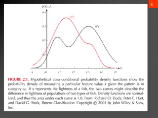
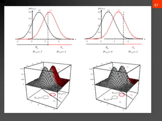
- 4. 3 ? Decision rule with only the prior information ? Decide ?1 if P(?1) > P(?2) otherwise decide ?2 ? Use of the class ©Cconditional information ? p(x | ?1) and p(x | ?2) describe the difference in lightness between populations of sea and salmon
- 5. 4
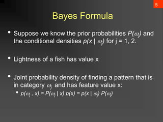
- 6. Bayes Formula ? Suppose we know the prior probabilities P(?j) and the conditional densities p(x | ?j) for j = 1, 2. ? Lightness of a fish has value x ? Joint probability density of finding a pattern that is in category ?j and has feature value x: ? p(?j , x) = P(?j | x) p(x) = p(x | ?j) P(?j) 5
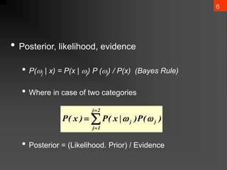
- 7. 6 ? Posterior, likelihood, evidence ? P(?j | x) = P(x | ?j) P (?j) / P(x) (Bayes Rule) ? Where in case of two categories ? Posterior = (Likelihood. Prior) / Evidence ? ? ? ? 2 j 1 j j j ) ( P ) | x ( P ) x ( P ? ?
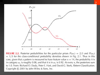
- 8. 7
- 9. 8 ? Decision given the posterior probabilities X is an observation for which: if P(?1 | x) > P(?2 | x) True state of nature = ?1 if P(?1 | x) < P(?2 | x) True state of nature = ?2 This rule minimizes average probability of error: ? ????? = ?Ī▐ Ī▐ ? ?????, ? ?? = ?Ī▐ Ī▐ ? ????? ? ? ? ?? p ????? ? = min[P(?1 | x), P(?2 | x) ] Decide ?1 if P(x | ?1) P (?1) > P(x | ?2) P (?2)
- 10. 9 2. Bayesian Decision Theory ©C Continuous Features ? Generalization of the preceding ideas 1. Use of more than one feature, vector X 2. Use more than two states of nature, c classes 3. Allowing actions other than deciding the state of nature 4. Introduce a loss of function which is more general than the probability of error
- 11. 10 ? Allowing actions other than classification primarily allows the possibility of rejection ? Rejection in the sense of abstention ? DonĪ»t make a decision if the alternatives are too close ? This must be tempered by the cost of indecision ? The loss function states how costly each action taken is
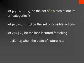
- 12. 11 Let {?1, ?2,ĪŁ, ?c} be the set of c states of nature (or Ī░categoriesĪ▒) Let {?1, ?2,ĪŁ, ?a} be the set of possible actions Let ?(?i | ?j) be the loss incurred for taking action ?i when the state of nature is ?j
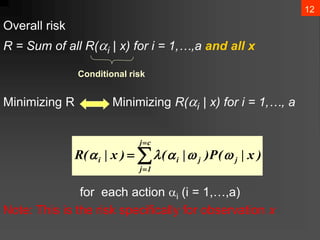
- 13. 12 Overall risk R = Sum of all R(?i | x) for i = 1,ĪŁ,a and all x Minimizing R Minimizing R(?i | x) for i = 1,ĪŁ, a for each action ?i (i = 1,ĪŁ,a) Note: This is the risk specifically for observation x Conditional risk ? ? ? ? c j 1 j j j i i ) x | ( P ) | ( ) x | ( R ? ? ? ? ?
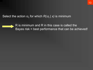
- 14. 13 Select the action ?i for which R(?i | x) is minimum R is minimum and R in this case is called the Bayes risk = best performance that can be achieved!
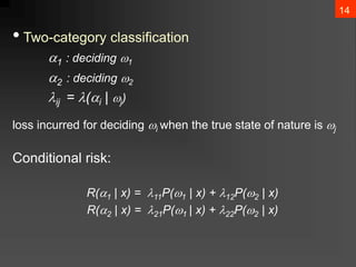
- 15. 14 ? Two-category classification ?1 : deciding ?1 ?2 : deciding ?2 ?ij = ?(?i | ?j) loss incurred for deciding ?i when the true state of nature is ?j Conditional risk: R(?1 | x) = ??11P(?1 | x) + ?12P(?2 | x) R(?2 | x) = ??21P(?1 | x) + ?22P(?2 | x)
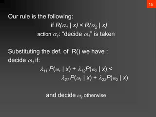
- 16. 15 Our rule is the following: if R(?1 | x) < R(?2 | x) action ?1: Ī░decide ?1Ī▒ is taken Substituting the def. of R() we have : decide ?1 if: ?11 P(?1 | x) + ?12P(?2 | x) < ?21 P(?1 | x) + ?22P(?2 | x) and decide ?2 otherwise
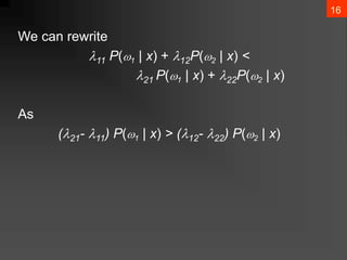
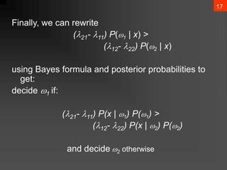
- 17. 16 We can rewrite ?11 P(?1 | x) + ?12P(?2 | x) < ?21 P(?1 | x) + ?22P(?2 | x) As (?21- ?11) P(?1 | x) > (?12- ?22) P(?2 | x)
- 18. 17 Finally, we can rewrite (?21- ?11) P(?1 | x) > (?12- ?22) P(?2 | x) using Bayes formula and posterior probabilities to get: decide ?1 if: (?21- ?11) P(x | ?1) P(?1) > (?12- ?22) P(x | ?2) P(?2) and decide ?2 otherwise
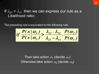
- 19. 18 If ?21 > ?11 then we can express our rule as a Likelihood ratio: The preceding rule is equivalent to the following rule: Then take action ?1 (decide ?1) Otherwise take action ?2 (decide ?2) ) ( P ) ( P . ) | x ( P ) | x ( P if 1 2 11 21 22 12 2 1 ? ? ? ? ? ? ? ? ? ? ?
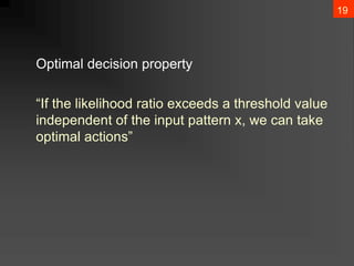
- 20. 19 Optimal decision property Ī░If the likelihood ratio exceeds a threshold value independent of the input pattern x, we can take optimal actionsĪ▒
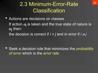
- 21. 20 2.3 Minimum-Error-Rate Classification ? Actions are decisions on classes If action ?i is taken and the true state of nature is ?j then: the decision is correct if i = j and in error if i ? j ? Seek a decision rule that minimizes the probability of error which is the error rate
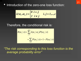
- 22. 21 ? Introduction of the zero-one loss function: Therefore, the conditional risk is: Ī░The risk corresponding to this loss function is the average probability errorĪ▒ c ,..., 1 j , i j i 1 j i 0 ) , ( j i ? ? ? ? ? ? ? ? ? ? ? ? ? ? ? ? ? ? ? i j i j c j j j j i i x P x P x P x R ) | ( 1 ) | ( ) | ( ) | ( ) | ( 1 ? ? ? ? ? ? ?
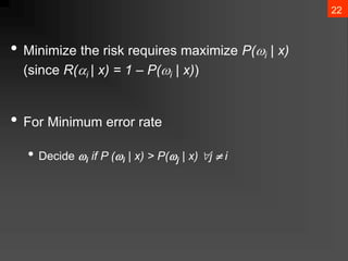
- 23. 22 ? Minimize the risk requires maximize P(?i | x) (since R(?i | x) = 1 ©C P(?i | x)) ? For Minimum error rate ? Decide ?i if P (?i | x) > P(?j | x) ?j ? i
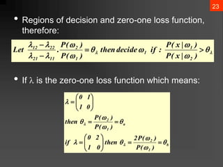
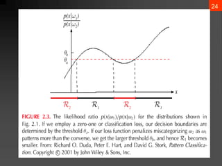
- 24. 23 ? Regions of decision and zero-one loss function, therefore: ? If ? is the zero-one loss function which means: b 1 2 a 1 2 ) ( P ) ( P 2 then 0 1 2 0 if ) ( P ) ( P then 0 1 1 0 ? ? ? ? ? ? ? ? ? ? ? ? ? ? ? ? ? ? ? ? ? ? ? ? ? ? ? ? ? ? ? ? ? ? ? ? ? ? ? ? ? ? ? ? ? ? ? ? ? ? ? ) | x ( P ) | x ( P : if decide then ) ( P ) ( P . Let 2 1 1 1 2 11 21 22 12
- 25. 24
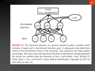
- 26. 25 4. Classifiers, Discriminant Functions, and Decision Surfaces ? The multi-category case ? Set of discriminant functions gi(x), i = 1,ĪŁ, c ? The classifier assigns a feature vector x to class ?i if: gi(x) > gj(x) ?j ? i
- 27. 26 ? Discriminant function gi(x) = P(?i | x) (max. discrimination corresponds to max. posterior!) gi(x) ? P(x | ?i) P(?i) gi(x) = ln P(x | ?i) + ln P(?i) (ln: natural logarithm!)
- 28. 27
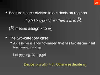
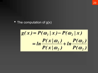
- 29. 28 ? Feature space divided into c decision regions if gi(x) > gj(x) ?j ? i then x is in Ri (Ri means assign x to ?i) ? The two-category case ? A classifier is a Ī░dichotomizerĪ▒ that has two discriminant functions g1 and g2 Let g(x) ? g1(x) ©C g2(x) Decide ?1 if g(x) > 0 ; Otherwise decide ?2
- 30. 29 ? The computation of g(x) ) ( P ) ( P ln ) | x ( P ) | x ( P ln ) x | ( P ) x | ( P ) x ( g 2 1 2 1 2 1 ? ? ? ? ? ? ? ? ? ?
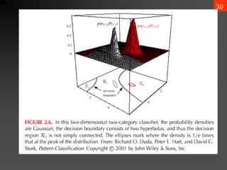
- 31. 30
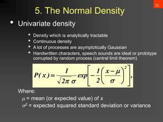
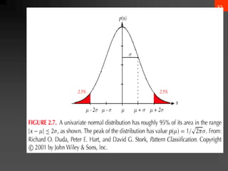
- 32. 31 5. The Normal Density ? Univariate density ? Density which is analytically tractable ? Continuous density ? A lot of processes are asymptotically Gaussian ? Handwritten characters, speech sounds are ideal or prototype corrupted by random process (central limit theorem) Where: ? = mean (or expected value) of x ?2 = expected squared standard deviation or variance , x 2 1 exp 2 1 ) x ( P 2 ? ? ? ? ? ? ? ? ? ? ? ? ? ? ? ? ? ? ? ? ?
- 33. 32
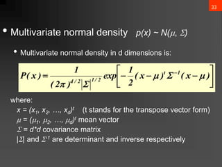
- 34. 33 ? Multivariate normal density p(x) ~ N(?, ?) ? Multivariate normal density in d dimensions is: where: x = (x1, x2, ĪŁ, xd)t (t stands for the transpose vector form) ? = (?1, ?2, ĪŁ, ?d)t mean vector ? = d*d covariance matrix |?| and ?-1 are determinant and inverse respectively ? ? ? ? ? ? ? ? ? ? ? ) x ( ) x ( 2 1 exp ) 2 ( 1 ) x ( P 1 t 2 / 1 2 / d ? ? ? ? ? ?
- 35. 34 ? = ?[x] = x?(x)?x ĪŲ = ?[(x??)(x??)t] = (x??)(x??)t?(x)?x ?? = ?[??] ??? = ?[(?? ? ??)(?? ? ??)]
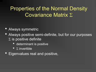
- 36. ? Always symmetric ? Always positive semi-definite, but for our purposes ? is positive definite ? determinant is positive ? ? invertible ? Eigenvalues real and positive, Properties of the Normal Density Covariance Matrix ?
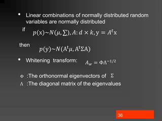
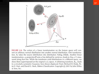
- 37. 36 ? Linear combinations of normally distributed random variables are normally distributed if then ? Whitening transform: :The orthonormal eigenvectors of :The diagonal matrix of the eigenvalues ?(x)~?(?, ĪŲ), ?: ? Ī┴ ?, y = ??x ?(y)~?(At?, At”▓A) ?? = ”Ą”½?1/2 ”Ą ”▓ ”½
- 38. 37 ?
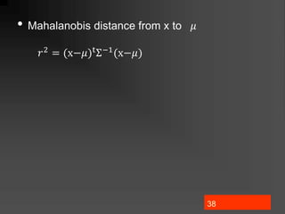
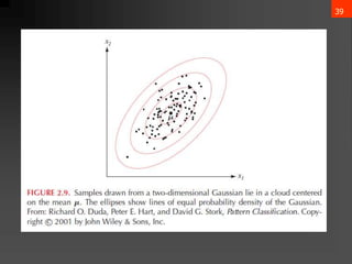
- 39. 38 ? Mahalanobis distance from x to ? ?2 = (x??)t”▓?1(x??)
- 40. 39 ?
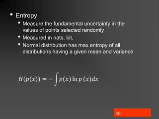
- 41. 40 ? Entropy ? Measure the fundamental uncertainty in the values of points selected randomly ? Measured in nats, bit, ? Normal distribution has max entropy of all distributions having a given mean and variance ?(?(?)) = ? ?(?) ln ? (?)??
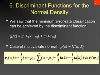
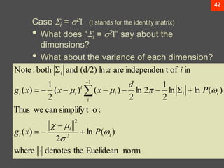
- 42. 41 6. Discriminant Functions for the Normal Density ? We saw that the minimum error-rate classification can be achieved by the discriminant function gi(x) = ln P(x | ?i) + ln P(?i) ? Case of multivariate normal p(x) ~ N(?, ?) ) ( P ln ln 2 1 2 ln 2 d ) x ( ) x ( 2 1 ) x ( g i i 1 i i t i i ? ? ? ? ? ? ? ? ? ? ? ? ? ?
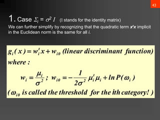
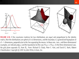
- 43. 42 Case ?i = ?2I (I stands for the identity matrix) ? What does Ī░?i = ?2IĪ▒ say about the dimensions? ? What about the variance of each dimension? norm Euclidean the denotes where ) ( ln 2 ) ( : o simplify t can we Thus ) ( ln ln 2 1 2 ln 2 ) ( ) ( 2 1 ) ( in of t independen are ln (d/2) and both : Note 2 2 1 i ? ? ? ? ? ? ? ? ? ? ? ? ? ? ? ? i i i i i i i t i i P x g P d x x x g i ? ? ? ? ? ? ? ? ?
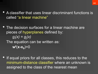
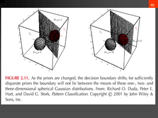
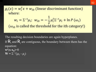
- 44. 43 1.Case ?i = ?2 I (I stands for the identity matrix) We can further simplify by recognizing that the quadratic term xtx implicit in the Euclidean norm is the same for all i. ) category! th the for threshold the called is ( ) ( P ln 2 1 w ; w : where function) nt discrimina (linear w x w ) x ( g 0 i i i t i 2 0 i 2 i i 0 i t i i i ? ? ? ? ? ? ? ? ? ? ? ? ?
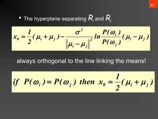
- 45. 44 ? A classifier that uses linear discriminant functions is called Ī░a linear machineĪ▒ ? The decision surfaces for a linear machine are pieces of hyperplanes defined by: gi(x) = gj(x) The equation can be written as: wt(x-x0)=0 ? If equal priors for all classes, this reduces to the minimum-distance classifier where an unknown is assigned to the class of the nearest mean
- 46. 45 ? The hyperplane separating Ri and Rj always orthogonal to the line linking the means! ) ( ) ( P ) ( P ln ) ( 2 1 x j i j i 2 j i 2 j i 0 ? ? ? ? ? ? ? ? ? ? ? ? ? ? ) ( 2 1 x then ) ( P ) ( P if j i 0 j i ? ? ? ? ? ? ?
- 47. 46
- 48. 47
- 49. 48
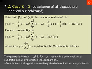
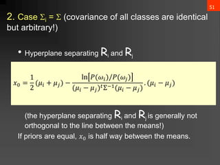
- 50. ? 2. Case ?i = ? (covariance of all classes are identical but arbitrary!) The quadratic form (? ? ??)? ĪŲ? ?1 (? ? ??) results in a sum involving a quadratic term xt ?-1x which is independent of i. After this term is dropped, the resulting discriminant function is again linear 49 Not?: both ”▓i an? (?/2) ln? ar? in??p?n??nt of ? in ??(?) = ? 1 2 (? ? ??)? ? ?1 (? ? ??) ? ? 2 ln 2 ? ? 1 2 ln ”▓? + ln ? (??) Thus w? can simplify to: ??(?) = ? 1 2 (? ? ??)? ? ?1 (? ? ??) + ln ? (??) wh?r? (? ? ??)? ? ?1 (? ? ??) ??not?s th? Mahalanobis ?istanc?
- 51. 50 ??(?) = ?? ? ? + ??0 (lin?ar ?iscriminant function) wh?r?: ?? = ??1??; ??0 = ? 1 2 ?? ? ??1?? + ln ? (??) (??0 is call?? th? thr?shol? for th? ith cat?gory!) The resulting decision boundaries are again hyperplanes. If Ri and Rj are contiguous, the boundary between them has the equation: wt(x-x0)=0 W = ??1(?? - ?j)
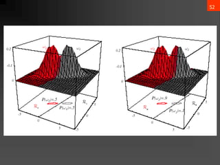
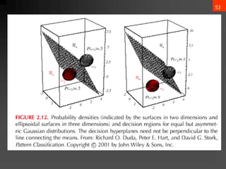
- 52. 51 2. Case ?i = ? (covariance of all classes are identical but arbitrary!) ? Hyperplane separating Ri and Rj (the hyperplane separating Ri and Rj is generally not orthogonal to the line between the means!) If priors are equal, ?0 is half way between the means. ?0 = 1 2 (?? + ??) ? ln ?(??)/?(??) (?? ? ??)?”▓?1(?? ? ??) . (?? ? ??)
- 53. 52
- 54. 53
- 55. 54
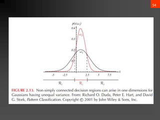
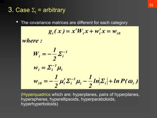
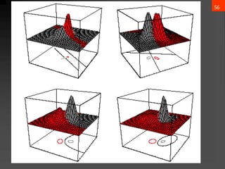
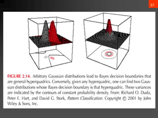
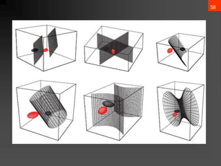
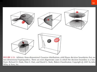
- 56. 55 3. Case ?i = arbitrary ? The covariance matrices are different for each category (Hyperquadrics which are: hyperplanes, pairs of hyperplanes, hyperspheres, hyperellipsoids, hyperparaboloids, hyperhyperboloids) ?? ? = ????? + ?? ? ? + ??0 ?????: Wi = ? 1 2 ”▓? ?1 wi = ”▓? ?1 ?? w?0 = ? 1 2 ?? ? ”▓? ?1 ?? ? 1 2 ln ”▓? + ln ? (??) ) ( P ln ln 2 1 2 1 w w 2 1 W : where w x w x W x ) x ( g i i i 1 i t i 0 i i 1 i i 1 i i 0 i t i i t i ? ? ? ? ? ? ? ? ? ? ? ? ? ? ? ? ? ? ? ? ?
- 57. 56
- 58. 57
- 59. 58
- 60. 59
- 61. 60
- 62. 61
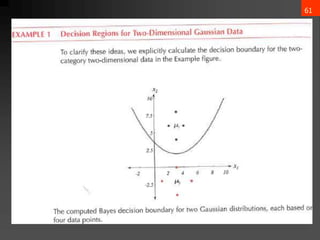
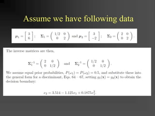
- 63. Assume we have following data
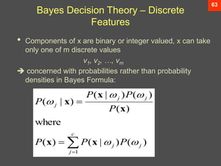
- 64. 63 Bayes Decision Theory ©C Discrete Features ? Components of x are binary or integer valued, x can take only one of m discrete values v1, v2, ĪŁ, vm ? concerned with probabilities rather than probability densities in Bayes Formula: ? ? ? ? c j j j j j j P P P P P P P 1 ) ( ) | ( ) ( where ) ( ) ( ) | ( ) | ( ? ? ? ? ? x x x x x
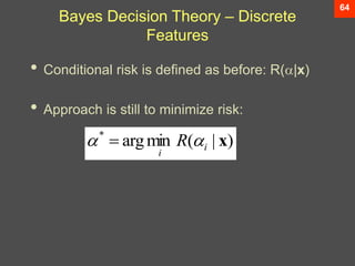
- 65. 64 Bayes Decision Theory ©C Discrete Features ? Conditional risk is defined as before: R(?|x) ? Approach is still to minimize risk: ) | ( min arg * x i i R ? ? ?
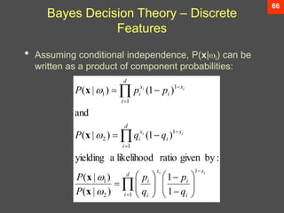
- 66. 65 Bayes Decision Theory ©C Discrete Features ? Case of independent binary features in 2 category problem Let x = [x1, x2, ĪŁ, xd ]t where each xi is either 0 or 1, with probabilities: pi = P(xi = 1 | ?1) qi = P(xi = 1 | ?2)
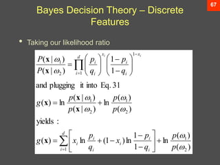
- 67. 66 Bayes Decision Theory ©C Discrete Features ? Assuming conditional independence, P(x|?i) can be written as a product of component probabilities: ? ? ? ? ? ? ? ? ? ? ? ? ? ? ? ? ? ? ? ? ? ? ? ? ? ? ? ? ? ? ? ? d i x i i x i i d i x i x i d i x i x i i i i i i i q p q p P P q q P p p P 1 1 2 1 1 1 2 1 1 1 1 1 ) | ( ) | ( : by given ratio likelihood a yielding ) 1 ( ) | ( and ) 1 ( ) | ( ? ? ? ? x x x x
- 68. 67 Bayes Decision Theory ©C Discrete Features ? Taking our likelihood ratio ) ( ) ( ln 1 1 ln ) 1 ( ln ) ( : yields ) ( ) ( ln ) | ( ) | ( ln ) ( 31 Eq. into it plugging and 1 1 ) | ( ) | ( 2 1 1 2 1 2 1 1 1 2 1 ? ? ? ? ? ? ? ? p p q p x q p x g p p p p g q p q p P P d i i i i i i i d i x i i x i i i i ? ? ? ? ? ? ? ? ? ? ? ? ? ? ? ? ? ? ? ? ? ? ? ? ? ? ? ? ? ? ? ? ? ? ? ? ? ? x x x x x x
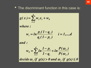
- 69. 68 ? The discriminant function in this case is: 0 g(x) if and 0 g(x) if decide ) ( P ) ( P ln q 1 p 1 ln w : and d ,..., 1 i ) p 1 ( q ) q 1 ( p ln w : where w x w ) x ( g 2 1 2 1 d 1 i i i 0 i i i i i 0 i d 1 i i ? ? ? ? ? ? ? ? ? ? ? ? ? ? ? ? ? ? ? ?
- 70. 69 Bayesian Belief Network ? Features ? Causal relationships ? Statistically independent ? Bayesian belief nets ? Causal networks ? Belief nets
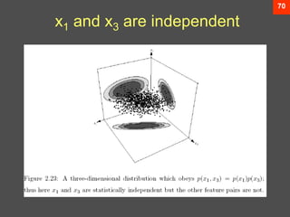
- 71. 70 x1 and x3 are independent
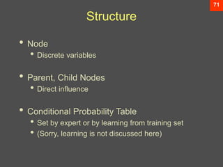
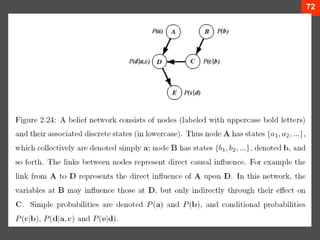
- 72. 71 Structure ? Node ? Discrete variables ? Parent, Child Nodes ? Direct influence ? Conditional Probability Table ? Set by expert or by learning from training set ? (Sorry, learning is not discussed here)
- 73. 72
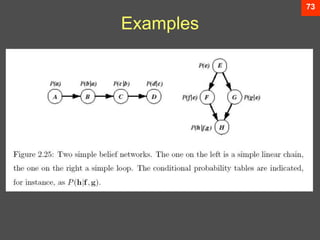
- 74. 73 Examples
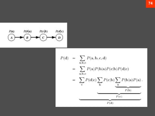
- 75. 74
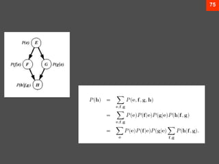
- 76. 75
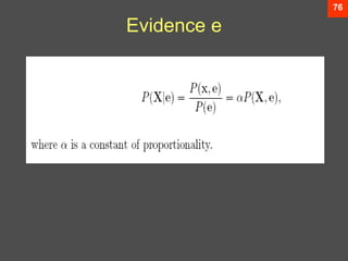
- 77. 76 Evidence e
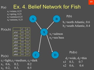
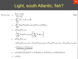
- 78. 77 Ex. 4. Belief Network for Fish A B X C D P(a) P(b) P(c|x) P(d|x) P(x|a,b) b1=north Atlantic, 0.6 b2=south Atlantic, 0.4 a1=winter, 0.25 a2=spring, 0.25 a3=summer,0.25 a4=autumn, 0.25 x1=salmon x2=sea bass d1=wide, d2=thin x1 0.3, 0.7 x2 0.6, 0.4 c1=light,c2=medium, c3=dark x1 0.6, 0.2, 0.2 x2 0.2, 0.3, 0.5 x1 x2 a1b1 0.5 0.5 a1b2 0.7 0.3 a2b1 0.6 0.4 a2b2 0.8 0.2 a3b1 0.4 0.6 a3b2 0.1 0.9 a4b1 0.2 0.8 a4b2 0.3 0.7
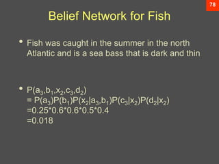
- 79. 78 Belief Network for Fish ? Fish was caught in the summer in the north Atlantic and is a sea bass that is dark and thin ? P(a3,b1,x2,c3,d2) = P(a3)P(b1)P(x2|a3,b1)P(c3|x2)P(d2|x2) =0.25*0.6*0.6*0.5*0.4 =0.018
- 80. Pattern Classification, Chapter 2 (Part 3) 79 Light, south Atlantic, fish?
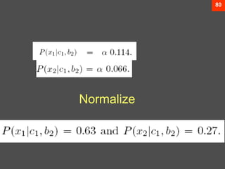
- 81. 80 Normalize
- 83. 82 Medical Application ? Medical diagnosis ? Uppermost nodes: biological agent ? (virus or bacteria) ? Intermediate nodes: diseases ? (flu or emphysema) ? Lowermost nodes: symptoms ? (high temperature or coughing) ? Finds the most likely disease or cause ? By entering measured values

![8
? Decision given the posterior probabilities
X is an observation for which:
if P(?1 | x) > P(?2 | x) True state of nature = ?1
if P(?1 | x) < P(?2 | x) True state of nature = ?2
This rule minimizes average probability of error:
? ????? =
?Ī▐
Ī▐
? ?????, ? ?? =
?Ī▐
Ī▐
? ????? ? ? ? ??
p ????? ? = min[P(?1 | x), P(?2 | x) ]
Decide ?1 if P(x | ?1) P (?1) > P(x | ?2) P (?2)](https://image.slidesharecdn.com/bayesiandecisiontheory1-240611161444-ca74f061/85/Bayesian-Decision-Theory-details-ML-pptx-9-320.jpg)
![34
? = ?[x] = x?(x)?x
ĪŲ = ?[(x??)(x??)t] = (x??)(x??)t?(x)?x
?? = ?[??]
??? = ?[(?? ? ??)(?? ? ??)]](https://image.slidesharecdn.com/bayesiandecisiontheory1-240611161444-ca74f061/85/Bayesian-Decision-Theory-details-ML-pptx-35-320.jpg)
![65
Bayes Decision Theory ©C Discrete
Features
? Case of independent binary features in 2
category problem
Let x = [x1, x2, ĪŁ, xd ]t where each xi is either 0
or 1, with probabilities:
pi = P(xi = 1 | ?1)
qi = P(xi = 1 | ?2)](https://image.slidesharecdn.com/bayesiandecisiontheory1-240611161444-ca74f061/85/Bayesian-Decision-Theory-details-ML-pptx-66-320.jpg)
