Bayesian His2011
- 1. Bayesian Methods in Machine Learning Mohammad Shazri mshazri@gmail.com shazri.shahrir@extolcorp.com
- 2. Sources âĒ Papers from Michael Tipping -Bayesian Inference: An introduction to Principles in Machine Learning âĒ Youtube from mathematicalmonk
- 3. approximate P(B|A) âĒ P(B|A)=f(A;w) âĶ.. A is the exemplars and w is the weights.|âgiven A, what is B?â. âĒ B and A usually relates as D= {A_n,B_n} from n=1 to N. âĒ Prior statements, possible to over-fit.
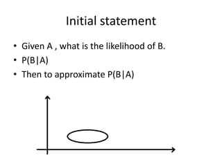
- 4. Initial statement âĒ Given A , what is the likelihood of B. âĒ P(B|A) âĒ Then to approximate P(B|A)
- 5. Setup and Model âĒ Setup; it is a supervised learning situation âĒ (1) Models/Basis* shape are normally distributed âĒ (2) confidence weights/tuneVar are independent. âĒ (3) there are precision tuners on basis+weights. Var and alpha âĒ (4) all are known except weights.
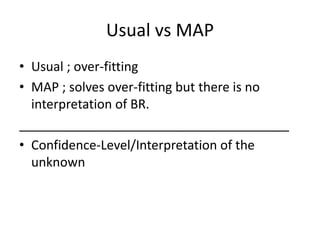
- 6. Usual vs MAP âĒ Usual ; over-fitting âĒ MAP ; solves over-fitting but there is no interpretation of BR. ______________________________________ âĒ Confidence-Level/Interpretation of the unknown
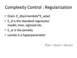
- 7. Complexity Control : Regularization âĒ E(w)= E_d(w)+lambda*E_w(w) âĒ E_d is the standard regression model, liner, sigmoid etc. âĒ E_w is the penalty âĒ Lamda is a hyperparameter
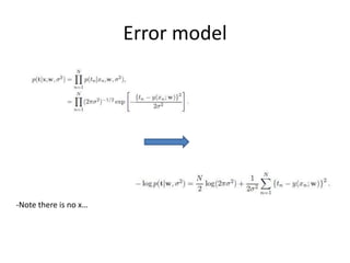
- 8. Error model -Note there is no xâĶ
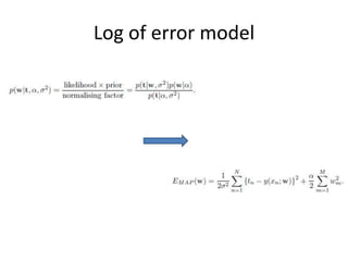
- 9. Log of error model
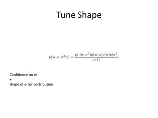
- 10. Tune Shape Confidence on w + shape of error contribution
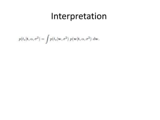
- 11. Interpretation
- 12. Lastly -Correspondence to NN -How we honestly manage complexity in Extol

