


![6-8
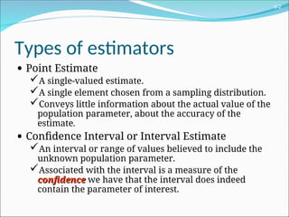
ŌĆó Consider the following statements:
’ā╝x = 550
ŌĆó A single-valued estimate that conveys little information
about the actual value of the population mean.
’ā╝We are 99% confident that ’üŁ is in the interval [449,551]
ŌĆó An interval estimate which locates the population mean
within a narrow interval, with a high level of confidence.
’ā╝We are 90% confident that ’üŁ is in the interval [400,700]
ŌĆó An interval estimate which locates the population mean
within a broader interval, with a lower level of confidence.](https://image.slidesharecdn.com/chapter7estimation-250131060630-24b5446f/85/Chapter-7-note-Estimation-ppt-biostatics-8-320.jpg)


More Related Content
Similar to Chapter 7 note Estimation.ppt biostatics (20)
Recently uploaded (20)


Chapter 7 note Estimation.ppt biostatics
- 2. 6-2 Types of estimators ŌĆó Point Estimate ’ā╝A single-valued estimate. ’ā╝A single element chosen from a sampling distribution. ’ā╝Conveys little information about the actual value of the population parameter, about the accuracy of the estimate. ŌĆó Confidence Interval or Interval Estimate ’ā╝An interval or range of values believed to include the unknown population parameter. ’ā╝Associated with the interval is a measure of the confidence confidence we have that the interval does indeed contain the parameter of interest.
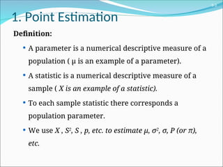
- 3. 6-3 1. Point Estimation Definition: ’éŚ A parameter is a numerical descriptive measure of a population ( ╬╝ is an example of a parameter). ’éŚ A statistic is a numerical descriptive measure of a sample ( X is an example of a statistic). ’éŚ To each sample statistic there corresponds a population parameter. ’éŚ We use X , S2 , S , p, etc. to estimate ╬╝, Žā2 , Žā, P (or ŽĆ), etc.
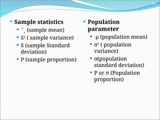
- 4. 6-4 ’éŚ Sample statistics ’éŚ ╦ē (sample mean) ’éŚ S2 ( sample variance) ’éŚ S (sample Standard deviation) ’éŚ P (sample proportion) ’éŚ Population parameter ’éŚ ╬╝ (population mean) ’éŚ Žā2 ( population variance) ’éŚ Žā(population standard deviation) ’éŚ P or ŽĆ (Population proportion) X
- 5. 6-5 Definition: ’éŚ A point estimate of some population parameter O is a single value ├ö of a sample statistic ’éŚ Sampling Distribution of Means ’éŚ one of the most fundamental concepts of statistical inference, and it has remarkable properties. ’éŚ Since it is a frequency distribution it has its own mean and standard deviation ’éŚ we shall use the notation for the standard deviation of the distribution. ’éŚ The standard deviation of the sampling distribution of means is called the standard error of the mean.
- 6. 6-6 ’éŚ Properties 1. The mean of the sampling distribution of means is the same as the population mean, ╬╝ . 2. The SD of the sampling distribution of means is Žā / n . ŌłÜ 3. The shape of the sampling distribution of means is approximately a normal curve, regardless of the shape of the population distribution and provided n is large enough (Central limit theorem).
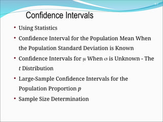
- 7. 6-7 ’ü¼ Using Statistics ’ü¼ Confidence Interval for the Population Mean When the Population Standard Deviation is Known ’ü¼ Confidence Intervals for ’üŁ When ’ü│ is Unknown - The t Distribution ’ü¼ Large-Sample Confidence Intervals for the Population Proportion p ’ü¼ Sample Size Determination Confidence Intervals
- 8. 6-8 ŌĆó Consider the following statements: ’ā╝x = 550 ŌĆó A single-valued estimate that conveys little information about the actual value of the population mean. ’ā╝We are 99% confident that ’üŁ is in the interval [449,551] ŌĆó An interval estimate which locates the population mean within a narrow interval, with a high level of confidence. ’ā╝We are 90% confident that ’üŁ is in the interval [400,700] ŌĆó An interval estimate which locates the population mean within a broader interval, with a lower level of confidence.
- 9. 6-9 A confidence interval or interval estimate is a range or interval of numbers believed to include an unknown population parameter. Associated with the interval is a measure of the confidence we have that the interval does indeed contain the parameter of interest. ŌĆó A confidence interval or interval estimate has two components: ’ā╝A range or interval of values ’ā╝An associated level of confidence
- 10. 6-10 ’ü¼ If the population distribution is normal, the sampling distribution of the mean is normal. ’éŚ If the sample is sufficiently large, regardless of the shape of the population distribution, the sampling distribution is normal (Central Limit Theorem). 95 . 0 96 . 1 96 . 1 or 95 . 0 96 . 1 96 . 1 : case either In ’ĆĮ ’āĘ ’āĖ ’āČ ’ā¦ ’ā© ’ā” ’Ć½ ’Ć╝ ’Ć╝ ’ĆŁ ’ĆĮ ’āĘ ’āĖ ’āČ ’ā¦ ’ā© ’ā” ’Ć½ ’Ć╝ ’Ć╝ ’ĆŁ n x n x P n x n P ’ü│ ’üŁ ’ü│ ’ü│ ’üŁ ’ü│ ’üŁ 4 3 2 1 0 -1 -2 -3 -4 0.4 0.3 0.2 0.1 0.0 z f(z) Standard Normal Distribution: 95% Interval
- 12. 6-12 Approximately 95% of the intervals around the sample mean can be expected to include the actual value of the population mean, ’üŁ. (When the sample mean falls within the 95% interval around the population mean.) *5% of such intervals around the sample mean can be expected not not to include the actual value of the population mean. (When the sample mean falls outside the 95% interval around the population mean.) x x’Ć½’Ć▒’Ć«’Ć╣’ĆČ’ü│ x’ĆŁ’Ć▒’Ć«’Ć╣’ĆČ’ü│ n x ’ü│ 96 . 1 ’é▒ 0.4 0.3 0.2 0.1 0.0 x f(x) Sampling Distribution of the Mean ’üŁ x x x x x x x x 2.5% 95% 2.5% ’üŁ ’ü│ ’ĆŁ 196 . n ’üŁ ’ü│ ’Ć½196 . n x x’Ć½’Ć▒’Ć«’Ć╣’ĆČ’ü│ x’ĆŁ’Ć▒’Ć«’Ć╣’ĆČ’ü│ * * p n u 95%
- 13. 6-13 Interpretation: a.Probabilistic: in repeated sampling, 100(1-╬▒)% of all intervals will include ╬╝ b.Practical: we are 100(1-╬▒)% confident that a interval contains ╬╝.
- 14. 6-14 A 95% confidence interval for ’üŁ when ’ü│ is known and sampling is done from a normal population, or a large sample is used: n x ’ü│ 96 . 1 ’é▒ The quantity is often called the margin of error or the sampling error. n ’ü│ 96 . 1 For example, if:n = 25 ’ü│’ĆĀ= 20 = 122 ’üø ’üØ 84 . 129 , 16 . 114 84 . 7 122 ) 4 )( 96 . 1 ( 122 25 20 96 . 1 122 96 . 1 ’ĆĮ ’é▒ ’ĆĮ ’é▒ ’ĆĮ ’é▒ ’ĆĮ ’é▒ n x ’ü│ A 95% confidence interval: x
- 16. 6-16 0.99 0.005 2.576 0.98 0.010 2.326 0.95 0.025 1.960 0.90 0.050 1.645 0.80 0.100 1.282 ( ) 1’ĆŁ ’üĪ ’üĪ 2 z’üĪ 2 z’üĪ 2 ( ) 1 ’ĆŁ ’üĪ ’ĆŁ z’üĪ 2 ’üĪ 2 ’üĪ 2
- 17. 6-17 When sampling from the same population, using a fixed sample size, the higher the confidence level, the wider the confidence interval. 5 4 3 2 1 0 -1 -2 -3 -4 -5 0.4 0.3 0.2 0.1 0.0 Z f(z) Stand ard Nor m al Distribution 80% Confidence Interval: x n ’é▒128 . ’ü│ 5 4 3 2 1 0 -1 -2 -3 -4 -5 0.4 0.3 0.2 0.1 0.0 Z f(z) Stand ard Nor m al Distributi on 95% Confidence Interval: x n ’é▒196 . ’ü│
- 18. 6-18 When sampling from the same population, using a fixed confidence level, the larger the sample size, n, the narrower the confidence interval. 0 .9 0 .8 0 .7 0 .6 0 .5 0 .4 0 .3 0 .2 0 .1 0 .0 x f(x) S am p ling D istrib utio n of the M e an 95% Confidence Interval: n = 40 0.4 0.3 0.2 0.1 0.0 x f(x) S am p ling D istrib utio n of the Me an 95% Confidence Interval: n = 20 0 .9 0 .8 0 .7 0 .6 0 .5 0 .4 0 .3 0 .2 0 .1 0 .0 x f(x) S am p ling D istrib utio n of the Me an 0 .4 0 .3 0 .2 0 .1 0 .0 x f(x) S am p ling D istrib utio n of the Me an 0 .9 0 .8 0 .7 0 .6 0 .5 0 .4 0 .3 0 .2 0 .1 0 .0 x f(x) S am p ling D istrib utio n of the Me an 0 .4 0 .3 0 .2 0 .1 0 .0 x f(x) S am p ling D istrib utio n of the Me an
- 19. 6-19 ’éŚ A physical therapist wished to estimate, with 99% confidence, the mean maximal strength of a particular muscle in a certain group of individuals. He assume that strength scores are approximately normally distributed with a variance of 144. A sample of 15 subjects who participated in the experiment yielded a mean of 84.3. What is 90% CI?
- 20. 6-20 Solution ╬▒ = 0.01ŌćÆ Z╬▒/2 = 2.58 Mean =84.3, n=15, Žā =12 84.3 ┬▒ 2.58(12/ ŌłÜ15) 84.3 ┬▒ 8.0 (76.3, 92.3) ŌćÆ ŌćÆ ŌćÆ We are 99% confident that the population mean is between 76.3 and 92.3.
- 21. 6-21 ŌĆó The t is a family of bell-shaped and symmetric distributions, one for each number of degree of freedom. ŌĆó The expected value of t is 0. ŌĆó For df > 2, the variance of t is df/(df-2). This is greater than 1, but approaches 1 as the number of degrees of freedom increases. The t is flatter and has fatter tails than does the standard normal. ŌĆó The t distribution approaches a standard normal as the number of degrees of freedom increases If the population standard deviation, ’ü│, is not known, replace ’ü│’ĆĀwith the sample standard deviation, s. If the population is normal, the resulting statistic: has a t distribution with (n - 1) degrees of freedom. t X s n ’ĆĮ ’ĆŁ ’üŁ Standard normal t, df = 20 t, df = 10 ’Ć░ ’üŁ
- 22. 6-22 A (1-’üĪ)100% confidence interval for ’üŁ when ’ü│ is not known (assuming a normally distributed population): where is the value of the t distribution with n-1 degrees of freedom that cuts off a tail area of to its right. t’üĪ 2 ’üĪ 2 n s t x 2 ’üĪ ’é▒
- 23. 6-23 df t0.100 t0.050 t0.025 t0.010 t0.005 --- ----- ----- ------ ------ ------ 1 3.078 6.314 12.706 31.821 63.657 2 1.886 2.920 4.303 6.965 9.925 3 1.638 2.353 3.182 4.541 5.841 4 1.533 2.132 2.776 3.747 4.604 5 1.476 2.015 2.571 3.365 4.032 6 1.440 1.943 2.447 3.143 3.707 7 1.415 1.895 2.365 2.998 3.499 8 1.397 1.860 2.306 2.896 3.355 9 1.383 1.833 2.262 2.821 3.250 10 1.372 1.812 2.228 2.764 3.169 11 1.363 1.796 2.201 2.718 3.106 12 1.356 1.782 2.179 2.681 3.055 13 1.350 1.771 2.160 2.650 3.012 14 1.345 1.761 2.145 2.624 2.977 15 1.341 1.753 2.131 2.602 2.947 16 1.337 1.746 2.120 2.583 2.921 17 1.333 1.740 2.110 2.567 2.898 18 1.330 1.734 2.101 2.552 2.878 19 1.328 1.729 2.093 2.539 2.861 20 1.325 1.725 2.086 2.528 2.845 21 1.323 1.721 2.080 2.518 2.831 22 1.321 1.717 2.074 2.508 2.819 23 1.319 1.714 2.069 2.500 2.807 24 1.318 1.711 2.064 2.492 2.797 25 1.316 1.708 2.060 2.485 2.787 26 1.315 1.706 2.056 2.479 2.779 27 1.314 1.703 2.052 2.473 2.771 28 1.313 1.701 2.048 2.467 2.763 29 1.311 1.699 2.045 2.462 2.756 30 1.310 1.697 2.042 2.457 2.750 40 1.303 1.684 2.021 2.423 2.704 60 1.296 1.671 2.000 2.390 2.660 120 1.289 1.658 1.980 2.358 2.617 1.282 1.645 1.960 2.326 2.576 ’éź 0 0 .4 0 .3 0 .2 0 .1 0 .0 t f(t) t D istrib utio n: d f=10 Area = 0.10 } Area = 0.10 } Area = 0.025 } Area = 0.025 } 1.372 -1.372 2.228 -2.228 Whenever ’ü│ is not known (and the population is assumed normal), the correct distribution to use is the t distribution with n-1 degrees of freedom. Note, however, that for large degrees of freedom, the t distribution is approximated well by the Z distribution.
- 24. 6-24 A study of hypoxemia during the immediate post-operative period reported the fractions of ideal weight for 11 patients who became severely hypoxemic during transfer to the recovery room. The mean is 1.51 and the standard deviation is 0.33. Estimate the 95% C.I. for the population mean fraction of ideal weight, where the population consists of hypoxemic patients similar to those in the study (The data is normally distributed, use ╬▒=0.05). Solution ŌĆó t╬▒/2, n-1 / = t 0.025,10 = 2.2281 1 . 51 ┬▒ 2 . 2281(0 . 33/’ā¢11) 1 . 51┬▒ 0 . 221 (1 . 289 ,1 . 731 ) ŌĆó We are 95% sure that the ╬╝ (1 . 289 ,1 . 731 ) population mean lies between 1.289 and 1.731
- 25. 6-25 Whenever ’ü│ is not known (and the population is assumed normal), the correct distribution to use is the t distribution with n-1 degrees of freedom. Note, however, that for large degrees of freedom, the t distribution is approximated well by the Z distribution. df t0.100 t0.050 t0.025 t0.010 t0.005 --- ----- ----- ------ ------ ------ 1 3.078 6.314 12.706 31.821 63.657 . . . . . . . . . . . . . . . . . . 120 1.289 1.658 1.980 2.358 2.617 1.282 1.645 1.960 2.326 2.576 ’éź
- 26. 6-26 n s z x 2 : for interval confidence )100% - (1 sample - large A ’üĪ ’üŁ ’üĪ ’é▒ Example 6-3: Example 6-3: An economist wants to estimate the average amount in checking accounts at banks in a given region. A random sample of 100 accounts gives x-bar = $357.60 and s = $140.00. Give a 95% confidence interval for ’üŁ, the average amount in any checking account at a bank in the given region. ’üø ’üØ x z s n ’é▒ ’ĆĮ ’é▒ ’ĆĮ ’é▒ ’ĆĮ 0 025 357.60 196 14000 100 357.60 27.44 33016,38504 . . . . .
- 27. 6-27 The estimator of the population proportion, , is the sample proportion, . If the sample size is large, p p p p p p pq n q = (1 - p) p p p n p n q ’Ćż ’Ćż ’Ćż ’Ćż ’Ćż ’Ćż has an approximately normal distribution, with E( ) = and V( ) = where . When the population proportion is unknown, use the estimated value, , to estimate the standard deviation of . For estimating , a sample is considered large enough when both an are greater than 5. , ’āŚ ’āŚ
- 28. 6-28 . p╠é - 1 = q╠é and , size), sample (the trials of number by the divided , sample, in the successes of number the to equal is , p╠é , proportion sample the where , proportion population for the interval confidence )100% - (1 sample - large A ╦å ╦å 2 ╦å n x : p n q p ╬▒ z p ’é▒ ’üĪ
- 29. 6-29 A marketing research firm wants to estimate the share that foreign companies have in the American market for certain products. A random sample of 100 consumers is obtained, and it is found that 34 people in the sample are users of foreign-made products; the rest are users of domestic products. Give a 95% confidence interval for the share of foreign products in this market. ’üø ’üØ ’Ćż ’Ćż ’Ćż . . ( . )( . ) . ( . )( . ) . . . , . p z pq n ’é▒ ’ĆĮ ’é▒ ’ĆĮ ’é▒ ’ĆĮ ’é▒ ’ĆĮ ’üĪ 2 0 34 196 0 34 0 66 100 0 34 196 0 04737 0 34 0 0928 0 2472 0 4328 Thus, the firm may be 95% confident that foreign manufacturers control anywhere from 24.72% to 43.28% of the market.
- 30. 6-30 The width of a confidence interval can be reduced only at the price of: ŌĆó a lower level of confidence, or ŌĆó a larger sample. ’üø ’üØ ’Ćż ’Ćż ’Ćż . . ( . )( . ) . ( . )( . ) . . . , . p z pq n ’é▒ ’ĆĮ ’é▒ ’ĆĮ ’é▒ ’ĆĮ ’é▒ ’ĆĮ ’üĪ 2 0 34 1645 0 34 0 66 100 0 34 1645 0 04737 0 34 0 07792 0 2621 0 4197 90% Confidence Interval ’üø ’üØ ’Ćż ’Ćż ’Ćż . . ( . )( . ) . ( . )( . ) . . . , . p z pq n ’é▒ ’ĆĮ ’é▒ ’ĆĮ ’é▒ ’ĆĮ ’é▒ ’ĆĮ ’üĪ 2 0 34 196 0 34 0 66 200 0 34 196 0 03350 0 34 0 0657 0 2743 0 4057 Sample Size, n = 200 Lower Level of Confidence Larger Sample Size
- 31. 6-31 ŌĆó How close do you want your sample estimate to be to the unknown parameter? (What is the desired bound, B?) ŌĆó What do you want the desired confidence level (1-’üĪ) to be so that the distance between your estimate and the parameter is less than or equal to B? ŌĆó What is your estimate of the variance (or standard deviation) of the population in question? Before determining the necessary sample size, three questions must be answered: n ’ü│ ’üŁ ’üĪ ’üĪ 2 z x : for Interval Confidence ) - (1 A : example For ’é▒
- 32. 6-32 ’üŁ Standard error of statistic Sample size = n Sample size = 2n Standard error of statistic The sample size determines the bound of a statistic, since the standard error of a statistic shrinks as the sample size increases:
- 33. 6-33
- 34. 6-34 A marketing research firm wants to conduct a survey to estimate the average amount spent on entertainment by each person visiting a popular resort. The people who plan the survey would like to determine the average amount spent by all people visiting the resort to within $120, with 95% confidence. From past operation of the resort, an estimate of the population standard deviation is s = $400. What is the minimum required sample size? n z B ’ĆĮ ’ĆĮ ’ĆĮ ’é╗ ’üĪ ’ü│ 2 2 2 2 2 2 2 1 96 400 120 42 684 43 ( . ) ( ) .
- 35. 6-35 The manufacturers of a sports car want to estimate the proportion of people in a given income bracket who are interested in the model. The company wants to know the population proportion, p, to within 0.01 with 99% confidence. Current company records indicate that the proportion p may be around 0.25. What is the minimum required sample size for this survey? n z pq B ’ĆĮ ’ĆĮ ’ĆĮ ’é╗ ’üĪ 2 2 2 2 2 2 576 025 0 75 010 124.42 125 . ( . )( . ) .