�ݺ�ߣ

Connectivity Methodology
Ver. 3.0
NRDC Sustainable Cities Team
Presenter: TL
July 15,2015

Outline
• Key updates
• Principles
• Input preparation
• Interim procedure
• Output result
• Evaluation of the Methodology

Key Updates
• Powerful ArcGIS (licensed authorization!)
• Overcome some constrains posed by KMZ preparation
• Generate random points
• Select eligible points
• Batch: python code
• Update of Cityname.xlsx file
• Skipping of sheet Random_Points
• Important annotation: the unit of average altitude is kilometers

Principles
• The process will…
• generate 1000 random points for each city;
• Increasing capacity is feasible
• allow us to choose 40 eligible points to measure the walking distances;
• Identify if the interim points meet the standard (od distance = 500m)
• Discard the points that do not meet the requirement
• Go back to the bank test if a new eligible point meet the requirement
• get average walking distances from the final 40 points;
• The process need to be…
• strictly random in point selecting
• accurate in calculating the distance
• comparable across all cities
• efficient

Input Preparation
• Google Earth Pro:
• citynameRND.kmz (Many thanks to Ning, Xiao, Judy, Chenzi, Danlu)
• Same setting requirement: degree (decimal)
• Microsoft Excel:
• cityname.xlsx
• (Random_Points_Value), Eligible_Points, (Eligible_Points_Raw), Square_Points, Distance
• ESRI ArcGIS 10.X:
• Manually geoprocessing
• Python stand-alone processing
• (Windows environment is strongly recommended!)
• VPN and good network

Interim procedure: RP gen and EP selection
• In ArcGIS:
• KMZ to Layer
• Feature class to feature class
• (transforming boundary polylines into polygons)
• Generate random points: CITYNAME_RP.dbf
• (confined by boundary polygons)
• Selecting eligible points: CITYNAME_EP.dbf
• Detailed procedure: consulting to the python file
• In Excel:
• Copy and paste fields: Name, Latitude, Longitude
• From CITYNAME_RP.dbf to sheet Random_Points_Value
• From CITYNAME_EP.dbf to sheet Eligible_Points_Value (1 st round EP)

Interim Procedure: Square Points
• In workbook Square_Points of Nanchang.xlsx:
• Fill value of Nanchang’s average altitude in the cell following Average
Altitude;

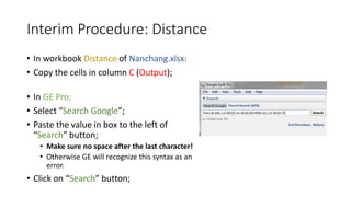
Interim Procedure: Distance
• In workbook Distance of Nanchang.xlsx:
• Copy the cells in column C (Output);
• In GE Pro;
• Select “Search Google”;
• Paste the value in box to the left of
“Search” button;
• Make sure no space after the last character!
• Otherwise GE will recognize this syntax as an
error.
• Click on “Search” button;

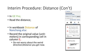
Interim Procedure: Distance (Con’t)
• In GE Pro;
• Read the distance;
• In workbook Distance of
Nanchang.xlsx:
• Record the original value (unit:
meters) in corresponding cell in
column E;
• Do not worry about the weird
direction/distance you get now.

• Check for reasonableness
• If the trip origination and trip
destination are approximately
located at the point eligible
points…
• You are lucky!

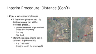
• Check for reasonableness
• If the trip origination and trip
destination are not at the
intended places…
• (distance between origination and
destination <> 500m)
• Too long
• Too short
• Mark the corresponding cell in
column I as problematic
• E.g. “*od<>500”
• (need to specify the error type?)

• Complete all 160 (4 square points of each eligible point * 40 eligible
points) entries
• Good luck!
• Review the notes for problematic results;
• You have made marks for each pair of eligible point and square point;
• Look at column I;
• Check if the note belongs to a problematic eligible point
• If more than 3/4 (including 3/4) direction/distance results of the eligible point
are marked as problematic, we need 2nd round of eligible points selecting;
• Clear all four results of the problematic eligible point in column E

Interim Procedure: 2nd round Eligible Points
• In workbook Eligible_Points of Nanchang.xlsx:
• Mark all problematic eligible points
• Find the first backup eligible points…
• Directly from Nanchang_RP layer in GE
• Manually replace the number of the problematic eligible point in column A with the one of
backup eligible point;
• Use a point from the back up list generated in 1st round
• Use a point from the back up list generated by ArcGIS
• (time saving)
• Repeat the Interim procedure: Distance
• If the back up point is still problematic, continue the process of finding new back up
eligible point.
• Finish the process when no problematic eligible points show up.

Output Result
• Save Nanchang.xlsx.
• The results will keep in workbook Distance;

Output Result
• Copy column B, C, and D to Nanchang_EP.csv;
• Save Nanchang_EP.csv;
• No need to copy column A;
• Copy column C, D, and E to Nanchang_Square.csv;
• Save Nanchang_Square.csv;
• No need to copy the rest columns;
• Import Nanchang_EP.csv and Nanchang_Square.csv to Nanchang.kmz in GE
Pro;
• Same procedure of importing Nanchang_RP.csv;
• Use different colors;
• Be sure to save to My Places;
• Save as Nanchang_Square.kmz;

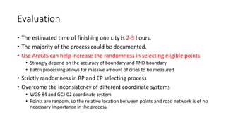
Evaluation
• The estimated time of finishing one city is 2-3 hours.
• The majority of the process could be documented.
• Use ArcGIS can help increase the randomness in selecting eligible points
• Strongly depend on the accuracy of boundary and RND boundary
• Batch processing allows for massive amount of cities to be measured
• Strictly randomness in RP and EP selecting process
• Overcome the inconsistency of different coordinate systems
• WGS-84 and GCJ-02 coordinate system
• Points are random, so the relative location between points and road network is of no
necessary importance in the process.

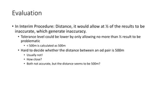
Evaluation
• In Interim Procedure: Distance, it would allow at ½ of the results to be
inaccurate, which generate inaccuracy.
• Tolerance level could be lower by only allowing no more than ½ result to be
problematic
• < 500m is calculated as 500m
• Hard to decide whether the distance between an od pair is 500m
• Usually not!
• How close?
• Both not accurate, but the distance seems to be 500m?

�ݺ�ߣ

Connectivity Methodology3.0

Recommended

More Related Content

What's hot (16)

Similar to Connectivity Methodology3.0 (20)

Connectivity Methodology3.0

Editor's Notes