際際滷

際際滷Share a Scribd company logo
Relations, Functions, and Matrices


                    Mathematical
                    Structures for
                  Computer Science
                               Chapter 4


    Section 4.6 息 2006 W.H. Freeman & Co.
     Copyright                               
   MSCS 際際滷s
                                                         Matrices   Relations, Functions and Matrices
Monday, March 29, 2010
Matrix

             Data about many kinds of problems can often be
              represented using a rectangular arrangement of values;
              such an arrangement is called a matrix.


             A is a matrix with two rows and three columns.
             The dimensions of the matrix are the number of rows
              and columns; here A is a 2  3 matrix.
             Elements of a matrix A are denoted by aij, where i is
              the row number of the element in the matrix and j is
              the column number.
             In the example matrix A, a23 = 8 because 8 is the
              element in row 2, column 3, of A.
    Section 4.6                         Matrices                      2
Monday, March 29, 2010
Example: Matrix

           The constraints of many problems are represented by
            the system of linear equations, e.g.:


     x + y = 70


     24x + 14y = 1180
        	

 The solution is x = 20, y = 50 (you can easily check
            that this is a solution).


             The matrix A is the matrix of coef鍖cients for this
              system of linear equations.

    Section 4.6                          Matrices                  3
Monday, March 29, 2010
Matrix
             If X = Y, then x = 3, y = 6, z = 2, and w = 0.


             We will often be interested in square matrices, in which the
              number of rows equals the number of columns.
             If A is an n  n square matrix, then the elements a11, a22, ... ,
              ann form the main diagonal of the matrix.
             If the corresponding elements match when we think of
              folding the matrix along the main diagonal, then the matrix
              is symmetric about the main diagonal.
             In a symmetric matrix, aij = aji.
    Section 4.6                              Matrices                        4
Monday, March 29, 2010
Matrix Operations

             Scalar multiplication calls for multiplying each entry
              of a matrix by a 鍖xed single number called a scalar.
              The result is a matrix with the same dimensions as the
              original matrix.
             The result of multiplying matrix A:


 by the scalar r = 3 is:


    Section 4.6                         Matrices                   5
Monday, March 29, 2010
Matrix Operations

             Addition of two matrices A and B is de鍖ned only
              when A and B have the same dimensions; then it is
              simply a matter of adding the corresponding elements.
             Formally, if A and B are both n  m matrices, then C
              = A + B is an n  m matrix with entries cij = aij + bij:


    Section 4.6                          Matrices                    6
Monday, March 29, 2010
Matrix Operations
             Subtraction of matrices is de鍖ned by


     A  B = A + ( l)B
             In a zero matrix, all entries are 0. If we add an n  m zero
              matrix, denoted by 0, to any n  m matrix A, the result is matrix
              A. We can symbolize this by the matrix equation:


     0+A=A
             If A and B are n  m matrices and r and s are scalars, the
              following matrix equations are true:


      A+B=B+A


     (A + B) + C = A + (B + C)


     r(A + B) = rA + rB


     (r + s)A = rA + sA


     r(sA) = (rs)A
        ! !         !      !       rA = Ar
    Section 4.6                               Matrices                            7
Monday, March 29, 2010
Matrix Operations

             Matrix multiplication is computed as A times B and
              denoted as A  B.
             Condition required for matrix multiplication: the
              number of columns in A must equal the number of
              rows in B. Thus we can compute A  B if A is an n  m
              matrix and B is an m  p matrix. The result is an n  p
              matrix.
             An entry in row i, column j of A  B is obtained by
              multiplying elements in row i of A by the
              corresponding elements in column j of B and adding
              the results. Formally, A  B = C, where


    Section 4.6                          Matrices                   8
Monday, March 29, 2010
Example: Matrix Multiplication

             To 鍖nd A  B = C for the following matrices:


             Similarly, doing the same for the other row, C is:


    Section 4.6                          Matrices                  9
Monday, March 29, 2010
Matrix Multiplication

             Compute A  B and B  A for the following matrices:


             Note that even if A and B have dimensions so that
              both A  B and B  A are de鍖ned, A  B need not equal
              B  A.


    Section 4.6                         Matrices                      10
Monday, March 29, 2010
Matrix Multiplication

             Where A, B, and C are matrices of appropriate
              dimensions and r and s are scalars, the following
              matrix equations are true (the notation A (B  C) is
              shorthand for A  (B  C)):


    A (B  C) = (A  B) C


    A (B + C) = A  B + A  C


    (A + B) C = A  C + B  C


    rA  sB = (rs)(A  B)
             The n  n matrix with 1s along the main diagonal and
              0s elsewhere is called the identity matrix, denoted by
              I. If we multiply I times any nn matrix A, we get A as
              the result. The equation is:


    IA=AI=A
    Section 4.6                          Matrices                  11
Monday, March 29, 2010
Matrix Multiplication Algorithm
        ALGORITHM MatrixMultiplication
        //computes n  p matrix A  B for n  m matrix A, m  p matrix B
        //stores result in C
        for i = 1 to n do
        	

 for j = 1 to p do


  C[i, j] = 0


  for k =1 to m do


      C[i, j] = C[i, j] + A[i, k] * B[k, j]


  end for
        	

 end for
        end for
        write out product matrix C
         If A and B are both n  n matrices, then there are (n3)

            multiplications and (n3) additions required. Overall complexity
            is (n3)
    Section 4.6                            Matrices                        12
Monday, March 29, 2010

More Related Content

CPSC 125 Ch 4 Sec 6

  • 1. Relations, Functions, and Matrices Mathematical Structures for Computer Science Chapter 4 Section 4.6 息 2006 W.H. Freeman & Co. Copyright MSCS 際際滷s Matrices Relations, Functions and Matrices Monday, March 29, 2010
  • 2. Matrix Data about many kinds of problems can often be represented using a rectangular arrangement of values; such an arrangement is called a matrix. A is a matrix with two rows and three columns. The dimensions of the matrix are the number of rows and columns; here A is a 2 3 matrix. Elements of a matrix A are denoted by aij, where i is the row number of the element in the matrix and j is the column number. In the example matrix A, a23 = 8 because 8 is the element in row 2, column 3, of A. Section 4.6 Matrices 2 Monday, March 29, 2010
  • 3. Example: Matrix The constraints of many problems are represented by the system of linear equations, e.g.: x + y = 70 24x + 14y = 1180 The solution is x = 20, y = 50 (you can easily check that this is a solution). The matrix A is the matrix of coef鍖cients for this system of linear equations. Section 4.6 Matrices 3 Monday, March 29, 2010
  • 4. Matrix If X = Y, then x = 3, y = 6, z = 2, and w = 0. We will often be interested in square matrices, in which the number of rows equals the number of columns. If A is an n n square matrix, then the elements a11, a22, ... , ann form the main diagonal of the matrix. If the corresponding elements match when we think of folding the matrix along the main diagonal, then the matrix is symmetric about the main diagonal. In a symmetric matrix, aij = aji. Section 4.6 Matrices 4 Monday, March 29, 2010
  • 5. Matrix Operations Scalar multiplication calls for multiplying each entry of a matrix by a 鍖xed single number called a scalar. The result is a matrix with the same dimensions as the original matrix. The result of multiplying matrix A: by the scalar r = 3 is: Section 4.6 Matrices 5 Monday, March 29, 2010
  • 6. Matrix Operations Addition of two matrices A and B is de鍖ned only when A and B have the same dimensions; then it is simply a matter of adding the corresponding elements. Formally, if A and B are both n m matrices, then C = A + B is an n m matrix with entries cij = aij + bij: Section 4.6 Matrices 6 Monday, March 29, 2010
  • 7. Matrix Operations Subtraction of matrices is de鍖ned by A B = A + ( l)B In a zero matrix, all entries are 0. If we add an n m zero matrix, denoted by 0, to any n m matrix A, the result is matrix A. We can symbolize this by the matrix equation: 0+A=A If A and B are n m matrices and r and s are scalars, the following matrix equations are true: A+B=B+A (A + B) + C = A + (B + C) r(A + B) = rA + rB (r + s)A = rA + sA r(sA) = (rs)A ! ! ! ! rA = Ar Section 4.6 Matrices 7 Monday, March 29, 2010
  • 8. Matrix Operations Matrix multiplication is computed as A times B and denoted as A B. Condition required for matrix multiplication: the number of columns in A must equal the number of rows in B. Thus we can compute A B if A is an n m matrix and B is an m p matrix. The result is an n p matrix. An entry in row i, column j of A B is obtained by multiplying elements in row i of A by the corresponding elements in column j of B and adding the results. Formally, A B = C, where Section 4.6 Matrices 8 Monday, March 29, 2010
  • 9. Example: Matrix Multiplication To 鍖nd A B = C for the following matrices: Similarly, doing the same for the other row, C is: Section 4.6 Matrices 9 Monday, March 29, 2010
  • 10. Matrix Multiplication Compute A B and B A for the following matrices: Note that even if A and B have dimensions so that both A B and B A are de鍖ned, A B need not equal B A. Section 4.6 Matrices 10 Monday, March 29, 2010
  • 11. Matrix Multiplication Where A, B, and C are matrices of appropriate dimensions and r and s are scalars, the following matrix equations are true (the notation A (B C) is shorthand for A (B C)): A (B C) = (A B) C A (B + C) = A B + A C (A + B) C = A C + B C rA sB = (rs)(A B) The n n matrix with 1s along the main diagonal and 0s elsewhere is called the identity matrix, denoted by I. If we multiply I times any nn matrix A, we get A as the result. The equation is: IA=AI=A Section 4.6 Matrices 11 Monday, March 29, 2010
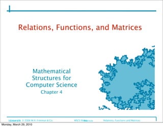
  • 12. Matrix Multiplication Algorithm ALGORITHM MatrixMultiplication //computes n p matrix A B for n m matrix A, m p matrix B //stores result in C for i = 1 to n do for j = 1 to p do C[i, j] = 0 for k =1 to m do C[i, j] = C[i, j] + A[i, k] * B[k, j] end for end for end for write out product matrix C If A and B are both n n matrices, then there are (n3) multiplications and (n3) additions required. Overall complexity is (n3) Section 4.6 Matrices 12 Monday, March 29, 2010