Data preprocessing in precision agriculture
- 1. Fall 2024-25 Precision Agriculture Dr. C. Moganapriya moganapriya.c@vit.ac.in
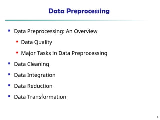
- 3. Data Preprocessing ’ü« Data Preprocessing: An Overview ’ü« Data Quality ’ü« Major Tasks in Data Preprocessing ’ü« Data Cleaning ’ü« Data Integration ’ü« Data Reduction ’ü« Data Transformation 3 3
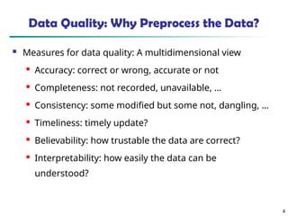
- 4. Data Quality: Why Preprocess the Data? ’ü« Measures for data quality: A multidimensional view ’ü« Accuracy: correct or wrong, accurate or not ’ü« Completeness: not recorded, unavailable, ŌĆ” ’ü« Consistency: some modified but some not, dangling, ŌĆ” ’ü« Timeliness: timely update? ’ü« Believability: how trustable the data are correct? ’ü« Interpretability: how easily the data can be understood? 4
- 5. Major Tasks in Data Preprocessing ’ü« Data cleaning ’ü« Data integration ’ü« Data reduction ’ü« Data transformation 5
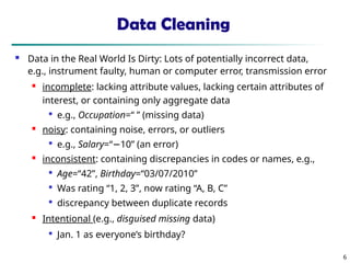
- 6. Data Cleaning ’ü« Data in the Real World Is Dirty: Lots of potentially incorrect data, e.g., instrument faulty, human or computer error, transmission error ’ü« incomplete: lacking attribute values, lacking certain attributes of interest, or containing only aggregate data ’ü« e.g., Occupation=ŌĆ£ ŌĆØ (missing data) ’ü« noisy: containing noise, errors, or outliers ’ü« e.g., Salary=ŌĆ£ŌłÆ10ŌĆØ (an error) ’ü« inconsistent: containing discrepancies in codes or names, e.g., ’ü« Age=ŌĆ£42ŌĆØ, Birthday=ŌĆ£03/07/2010ŌĆØ ’ü« Was rating ŌĆ£1, 2, 3ŌĆØ, now rating ŌĆ£A, B, CŌĆØ ’ü« discrepancy between duplicate records ’ü« Intentional (e.g., disguised missing data) ’ü« Jan. 1 as everyoneŌĆÖs birthday? 6
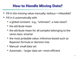
- 7. How to Handle Missing Data? ’ü« Fill in the missing value manually: tedious + infeasible? ’ü« Fill in it automatically with ’ü« a global constant : e.g., ŌĆ£unknownŌĆØ, a new class?! ’ü« the attribute mean ’ü« the attribute mean for all samples belonging to the same class: smarter ’ü« the most probable value: inference-based such as Bayesian formula or decision tree ’ü« Manual- small data set ’ü« Automatic ŌĆō larger data set ŌĆōmore efficient 7
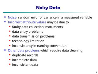
- 8. 8 Noisy Data ’ü« Noise: random error or variance in a measured variable ’ü« Incorrect attribute values may be due to ’ü« faulty data collection instruments ’ü« data entry problems ’ü« data transmission problems ’ü« technology limitation ’ü« inconsistency in naming convention ’ü« Other data problems which require data cleaning ’ü« duplicate records ’ü« incomplete data ’ü« inconsistent data
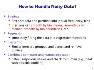
- 9. How to Handle Noisy Data? ’ü« Binning ’ü« first sort data and partition into (equal-frequency) bins ’ü« then one can smooth by bin means, smooth by bin median, smooth by bin boundaries, etc. ’ü« Regression ’ü« smooth by fitting the data into regression functions ’ü« Clustering ’ü« Similar item are grouped and detect and remove outliers ’ü« Combined computer and human inspection ’ü« detect suspicious values and check by human (e.g., deal with possible outliers) 9
- 10. Data Integration ’ü« Data integration: ’ü« Combines data from multiple heterogeneous sources into a coherent store ’ü« 2 types ’ü« Tight Coupling ’ü« Data is combined together into a physical location ’ü« Loose coupling ’ü« only an interface is created, and the data is combined through the interface and accessed through the interface ’ü« data reminds in actual database only 10 10
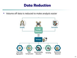
- 11. Data Reduction ’ü« Volume off data is reduced to make analysis easier 11 11
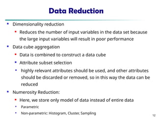
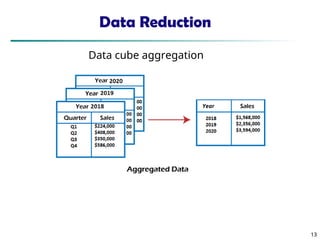
- 12. Data Reduction ’ü« Dimensionality reduction ’ü« Reduces the number of input variables in the data set because the large input variables will result in poor performance ’ü« Data cube aggregation ’ü« Data is combined to construct a data cube ’ü« Attribute subset selection ’ü« highly relevant attributes should be used, and other attributes should be discarded or removed, so in this way the data can be reduced ’ü« Numerosity Reduction: ’ü« Here, we store only model of data instead of entire data ’ü« Parametric ’ü« Non-parametric: Histogram, Cluster, Sampling 12 12
- 13. Data Reduction 13 13 Data cube aggregation
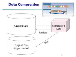
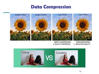
- 14. Data Compression 14 Original Data Compressed Data lossless Original Data Approximated lossy
- 16. Data Transformation ’ü« Data is transformed into appropriate form suitable for mining process ’ü« There are 4 methods in data transformation ’ü« 1. Normalization ’ü« 2. Attribute selection ’ü« 3. Discretization ’ü« 4. Concept hierarchy generation 1. Normalization Normalization is done in order to scale the data values in a specified range For example, -1.0 to + 1.0 or 0 to 1 16 16
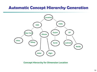
- 17. Data Transformation 2. Attribute selection New attributes are created using older ones 3. Discretization Raw values are replaced by interval values 4. Concept hierarchy generation Attributes are converted from low level to the higher level Example: city to country 17 17
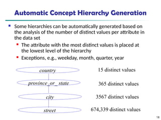
- 18. Automatic Concept Hierarchy Generation ’ü« Some hierarchies can be automatically generated based on the analysis of the number of distinct values per attribute in the data set ’ü« The attribute with the most distinct values is placed at the lowest level of the hierarchy ’ü« Exceptions, e.g., weekday, month, quarter, year 18 country province_or_ state city street 15 distinct values 365 distinct values 3567 distinct values 674,339 distinct values
- 19. Automatic Concept Hierarchy Generation 19
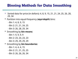
- 20. Binning Methods for Data Smoothing ’ü▒ Sorted data for price (in dollars): 4, 8, 9, 15, 21, 21, 24, 25, 26, 28, 29, 34 * Partition into equal-frequency (equi-depth) bins: - Bin 1: 4, 8, 9, 15 - Bin 2: 21, 21, 24, 25 - Bin 3: 26, 28, 29, 34 * Smoothing by bin means: - Bin 1: 9, 9, 9, 9 - Bin 2: 23, 23, 23, 23 - Bin 3: 29, 29, 29, 29 * Smoothing by bin boundaries: - Bin 1: 4, 4, 4, 15 - Bin 2: 21, 21, 25, 25 - Bin 3: 26, 26, 26, 34 20
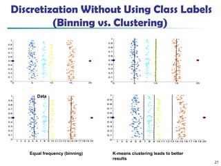
- 21. 21 Discretization Without Using Class Labels (Binning vs. Clustering) Data Equal interval width (binning) Equal frequency (binning) K-means clustering leads to better results
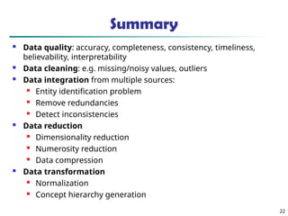
- 22. Summary ’ü« Data quality: accuracy, completeness, consistency, timeliness, believability, interpretability ’ü« Data cleaning: e.g. missing/noisy values, outliers ’ü« Data integration from multiple sources: ’ü« Entity identification problem ’ü« Remove redundancies ’ü« Detect inconsistencies ’ü« Data reduction ’ü« Dimensionality reduction ’ü« Numerosity reduction ’ü« Data compression ’ü« Data transformation ’ü« Normalization ’ü« Concept hierarchy generation 22

