�ݺ�ߣ

DECISION TREE
Bayesian Approach

DR. KALPNA SHARMA,
D E PA R T M E N T O F M AT H E M AT I C S
M A N I PA L U N I V E R S I T Y J A I P U R

1

DECISION TREES

 A decision tree is a chronological representation of the
decision problem.
 Each decision tree has two types of nodes; round nodes
correspond to the states of nature while square nodes
correspond to the decision alternatives.
 The branches leaving each round node represent the
different states of nature while the branches leaving each
square node represent the different decision alternatives.
 At the end of each limb of a tree are the payoffs attained
from the series of branches making up that limb.

2
DR. KALPNA SHARMA, DEPARTMENT OF MATHEMATICS, MANIPAL
UNIVERSITY JAIPUR

FIVE STEPS TO
DECISION TREE ANALYSIS

1. Define the problem.
2. Structure or draw the decision tree.
3. Assign probabilities to the states of nature.
4. Estimate payoffs for each possible combination of
alternatives and states of nature.
5. Solve the problem by computing expected
monetary values (EMVs) for each state of nature
node.

3
UNIVERSITY JAIPUR

EXAMPLE

A developer must decide how large a luxury
condominium complex to build – small, medium, or
large. The profitability of this complex depends upon
the future level of demand for the complex’s
condominiums.

4
UNIVERSITY JAIPUR

ELEMENTS OF DECISION THEORY

States of nature: The states of nature could be defined as low
demand and high demand.
Alternatives: Developer could decide to build a small, medium,
or large condominium complex.
Payoffs: The profit for each alternative under each potential
state of nature is going to be determined.

We develop different models for this problem on the following
slides.

5
UNIVERSITY JAIPUR

PAYOFF TABLE

THIS IS A PROFIT PAYOFF TABLE
States of Nature
Alternatives Low High
Small 8 8
Medium 5 15
Large -11 22

(payoffs in millions)
DR. KALPNA SHARMA,
DEPARTMENT OF MATHEMATICS,
MANIPAL UNIVERSITY JAIPUR
6

DECISION TREE

8

8

5

Medium Complex
15

-11

7
22
UNIVERSITY JAIPUR

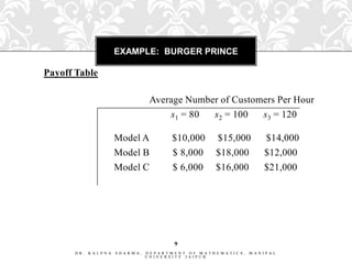
EXAMPLE: BURGER PRINCE

Burger Prince Restaurant is contemplating
opening a new restaurant on Main Street. It has three
different models, each with a different seating capacity.
Burger Prince estimates that the average number of
customers per hour will be 80, 100, or 120. The payoff
table (profits) for the three models is on the next slide.

8
UNIVERSITY JAIPUR


Payoff Table

Average Number of Customers Per Hour
s1 = 80 s2 = 100 s3 = 120

Model A $10,000 $15,000 $14,000
Model B $ 8,000 $18,000 $12,000
Model C $ 6,000 $16,000 $21,000

9
UNIVERSITY JAIPUR


Expected Value Approach
Calculate the expected value for each decision.
The decision tree on the next slide can assist in this
calculation. Here d1, d2, d3 represent the decision alternatives
of models A, B, C, and s1, s2, s3 represent the states of nature
of 80, 100, and 120.

10
UNIVERSITY JAIPUR

EXAMPLE: BURGER PRINCE Payoffs
s1 .4
10,000
s2 .2
2 s3 15,000
.4
d1 14,000
s1 .4
d2 8,000
1 s2 .2
3 18,000
d3 s3 .4
12,000
s1 .4
6,000
s2 .2
4 16,000
s3
.4
21,000
11
UNIVERSITY JAIPUR


Expected Value For Each Decision

EMV = .4(10,000) + .2(15,000) + .4(14,000)
= $12,600
d1 2
Model A
EMV = .4(8,000) + .2(18,000) + .4(12,000)
Model B d2 = $11,600
1 3

d3 EMV = .4(6,000) + .2(16,000) + .4(21,000)
Model C
= $14,000
4

Choose the model with largest EV, Model C.
DR. KALPNA SHARMA,
12
DEPARTMENT OF MATHEMATICS, MANIPAL
UNIVERSITY JAIPUR

EXAMPLE PROBLEM:
THOMPSON LUMBER COMPANY

Thompson Lumber Company is trying to decide whether to
expand its product line by manufacturing and marketing a new
product which is “backyard storage sheds.”
The courses of action that may be chosen include:
(1) large plant to manufacture storage sheds,
(2) small plant to manufacture storage sheds, or
(3) build no plant at all.

13
UNIVERSITY JAIPUR

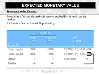
THOMPSON LUMBER COMPANY

Probability 0.5 0.5
14
UNIVERSITY JAIPUR

EXPECTED MONETARY VALUE
Thompson Lumber Company

Probability of favorable market is same as probability of unfavorable
market.
Each state of nature has a 0.50 probability.

15
UNIVERSITY JAIPUR

CALCULATING THE EVPI

Best outcome for state of nature "favorable market" is
"build a large plant" with a payoff of $200,000.
Best outcome for state of nature "unfavorable market"
is "do nothing," with payoff of $0.
Therefore, Expected profit with perfect information
EPPI = ($200,000)(0.50) + ($0)(0.50) = $ 100,000
If one had perfect information, an average payoff of
$100,000 could be achieved in the long run.
However, the maximum EMV (EV BEST) or expected
value without perfect information, is $40,000.
16
Therefore, EVPI = $100,000 - $40,000 = $60,000.
DR. KALPNA SHARMA, DEPARTMENT OF MATHEMATICS,
UNIVERSITY JAIPUR
MANIPAL

TO TEST OR NOT TO TEST

Often, companies have the option to perform market
tests/surveys, usually at a price, to get additional
information prior to making decisions.
However, some interesting questions need to be
answered before this decision is made:
How will the test results be combined with prior information?
How much should you be willing to pay to test?

The good news is that Bayes’ Theorem can be used to
combine the information, and we can use our decision
tree to find EVSI, the Expected Value of Sample
Information.
In order to perform these calculations, we first need to
know how reliable the potential test may be.
17
UNIVERSITY JAIPUR

MARKET SURVEY RELIABILITY IN PREDICTING
ACTUAL STATES OF NATURE

Assuming that the above information is available, we
can combine these conditional probabilities with our
prior probabilities using Bayes’ Theorem.
18
UNIVERSITY JAIPUR

MARKET SURVEY RELIABILITY IN PREDICTING ACTUAL
STATES OF NATURE

19
UNIVERSITY JAIPUR

PROBABILITY REVISIONS GIVEN
POSITIVE SURVEY

Alternatively, the following table will produce the same results:

20
UNIVERSITY JAIPUR

PROBABILITY REVISIONS GIVEN
NEGATIVE SURVEY

21
UNIVERSITY JAIPUR

PLACING POSTERIOR
PROBABILITIES ON THE DECISION
TREE
The bottom of the tree is the “no test” part of the analysis;
therefore, the prior probabilities are assigned to these events.
P(favorable market) = P(FM) = 0.5
P(unfavorable market) = P(UM) = 0.5
The calculations here will be identical to the EMV
calculations performed without a decision tree.

The top of the tree is the “test” part of the analysis; therefore,
the posterior probabilities are assigned to these events.

DR. KALPNA SHARMA,
DEPARTMENT OF MATHEMATICS,
MANIPAL UNIVERSITY JAIPUR
22

DECISION TREES FOR TEST/NO TEST MULTI-STAGE
DECISION PROBLEMS

23
UNIVERSITY JAIPUR

DECISION TREE SOLUTION
Thompson Lumber Company

24
UNIVERSITY JAIPUR

IN-CLASS PROBLEM 3
Leo can purchase a historic home for $200,000 or land in a growing area for
$50,000. There is a 60% chance the economy will grow and a 40% change it will
not. If it grows, the historic home will appreciate in value by 15% yielding a
$30,00 profit. If it does not grow, the profit is only $10,000. If Leo purchases the
land he will hold it for 1 year to assess the economic growth. If the economy grew
during the first year, there is an 80% chance it will continue to grow. If it did not
grow during the first year, there is a 30% chance it will grow in the next 4 years.
After a year, if the economy grew, Leo will decide either to build and sell a house
or simply sell the land. It will cost Leo $75,000 to build a house that will sell for a
profit of $55,000 if the economy grows, or $15,000 if it does not grow. Leo can
sell the land for a profit of $15,000. If, after a year, the economy does not grow,
Leo will either develop the land, which will cost $75,000, or sell the land for a
profit of $5,000. If he develops the land and the economy begins to grow, he will
make $45,000. If he develops the land and the economy does not grow, he will
make $5,000.
25
UNIVERSITY JAIPUR

IN-CLASS
PROBLEM 3:
2 SOLUTION Economy grows (.6)

No growth (.4)

Purchase
Economy grows
historic home
(.8)
Build house 6
No growth (.2)
1 4
Sell
Economy grows land
Purchase land (.6)

3 Economy grows
(.3)

No growth (.4) Develop land 7
No growth (.7)

5
Sell land

26
UNIVERSITY JAIPUR

IN-CLASS PROBLEM 3: SOLUTION

$22,000 Economy grows (.6) $30,000
2
No growth (.4)
$10,000

Purchase
Economy grows
historic home $55,000
$47,000 (.8)
Build house 6
$35,000 No growth (.2) $15,000
1 4
Sell $15,000
Economy grows $47,000
land
Purchase land (.6)

3 Economy grows
$45,000
$17,000 (.3)
$35,000
No growth (.4) Develop land 7
No growth (.7) $5,000

5
Sell land $5,000
$17,000
27
UNIVERSITY JAIPUR

SIMPLE EXAMPLE: UTILITY THEORY

Let’s say you were offered $2,000,000 right now on a chance to win
$5,000,000. The $5,000,000 is won only if you flip a coin and get
tails. If you get heads you lose and get $0. What should you do?
$2,000,000

$0
Heads
(0.5)

Tails
(0.5)

$5,000,000
28
UNIVERSITY JAIPUR

Decision Trees

29
UNIVERSITY JAIPUR

Planning Tool

30
UNIVERSITY JAIPUR

DECISION TREES

Enable a business to quantify decision making
Useful when the outcomes are uncertain
Places a numerical value on likely or potential
outcomes
Allows comparison of different possible decisions
to be made

31
UNIVERSITY JAIPUR

DECISION TREES

Limitations:
How accurate is the data used in the construction of the tree?
How reliable are the estimates of the probabilities?
Data may be historical – does this data relate to real time?
Necessity of factoring in the qualitative factors – human
resources, motivation, reaction, relations with suppliers and
other stakeholders

32
UNIVERSITY JAIPUR

Process

33
UNIVERSITY JAIPUR

THE PROCESS

Economic growth rises Expected outcome
0.7 £300,000

Expand by opening new outlet
Economic growth declines Expected outcome
-£500,000
0.3

Maintain current status
£0

The circle denotes the point where different outcomes could occur. The
estimates of the probability and the knowledge of the expected outcome
allow theadenotes the pointuncertainty is maintain thethe economy – quo! This wouldcontinuesoutcome of is:
A square firm to make a calculation of the likely return. In this example it
where a decision is made, In this example, a business is contemplating
There is also the outlet. The nothing and the state of current status if the economy have an to grow
opening new option to do
£0.
healthily the option is estimated to yield profits of £300,000. However, if the economy fails to grow as
Economicthe potentialrises:estimated£300,000 = £210,000
expected, growth loss is 0.7 x at £500,000.

Economic growth declines: 0.3 x £500,000 = -£150,000
34
The calculation would suggest it is wise to go ahead with the decision ( a net
‘benefit’ figure. ofA +£60,000)A , U N IPVAERRTSMI E Y TJ A IFP U RA T H E M A T I C S , M A N I P A L
DR K LPNA SHARM DE
T
N O M

The Process
Economic growth rises Expected outcome
0.5 £300,000

Expand by opening new outlet
Economic growth declines Expected outcome
-£500,000
0.5

Maintain current status
£0

Look what happens however if the probabilities change. If the firm is unsure of the
potential for growth, it might estimate it at 50:50. In this case the outcomes will be:
Economic growth rises: 0.5 x £300,000 = £150,000
Economic growth declines: 0.5 x -£500,000 = -£250,000
35
In this instance,D the A L P N benefit A , D E P A R T M E N T – Fthe TdecisionS ,looksPless favourable!
R. K
net A S H A R M is -£100,000 O M A H E M A T I C M A N I A L
UNIVERSITY JAIPUR

Advantages

36
UNIVERSITY JAIPUR

Disadvantages

37
UNIVERSITY JAIPUR

38
UNIVERSITY JAIPUR

�ݺ�ߣ

Decision tree

More Related Content

Decision tree