DerivaciÃģn 1.
Download as pptx, pdf0 likes148 views

The document defines the derivative of a function as the limit of the average rate of change of the function over an interval as the interval approaches zero. It provides examples of calculating the derivative of various functions, including the velocity and acceleration of the function s(t)=t^3 - 2t^2. The derivative of s(t) is 3t^2 - 4t, the velocity is 3t^2 - 4t, and the acceleration is 6t - 4. Formulas are provided for taking the derivative of various functions.

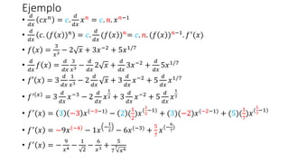
![Ejemplo
âĒ
ð
ððĨ
ð. (ð ðĨ )ð
= ð.
ð
ððĨ
(ð ðĨ )ð
= ð. ð. (ð ðĨ )ðâ1
. ðâē
(ðĨ)
âĒ â ðĨ = ð(ð ðĨ ); ð ðĨ = 3ðĨ6
; ð ðĨ = ðĨ3
+ ðĨ2
+ 1
âĒ ðâē ðĨ = 18ðĨ5
; ð ðĨ = 3ðĨ2
+ 2ðĨ
âĒ â ðĨ = 3(ðĨ3
+ ðĨ2
+ 1)6
; â ðĨ = ð(ð ðĨ )ð
âĒ ââē ðĨ
= c. ð. (ð ðĨ )ðâ1
. ðâē
(ðĨ)
âĒ â ðĨ = ð[ð ðĨ ]ð
âĒ ââē ðĨ
= ðâē
ð ðĨ . ðâē
(ðĨ)
âĒ
ð
ððĨ
â ðĨ =
ð
ððĨ
( 3 ðĨ3
+ ðĨ2
+ 1 6
)
âĒ ââē ðĨ = 3.6 ðĨ3 + ðĨ2 + 1 6â1. (3ðĨ2 + 2ðĨ)
âĒ ââē
ðĨ = 18 ðĨ3
+ ðĨ2
+ 1 5
. (3ðĨ2
+ 2ðĨ)](https://image.slidesharecdn.com/derivacin1-211201152208/85/Derivacion-1-24-320.jpg)
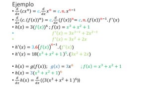
![Ejemplo
âĒ â ðĨ = ð[ð ðĨ ]ð
âĒ ââē(ðĨ) = ðâē ð ðĨ . ðâē(ðĨ)
âĒ â ðĨ =
4
(2ðĨ3 + 3ðĨ4 â ðĨ2)3
âĒ f ðĨ = 2ðĨ3 + 3ðĨ4 â ðĨ2 ; g x =
4
ðĨ3 = ðĨ
3
4
âĒ ðâē ðĨ = 6ðĨ2 + 12ðĨ3 â 2ðĨ ; ðâē ðĨ =
3
4
. ðĨ(
3
4
â1)
âĒ ðâē ðĨ = 6ðĨ2 + 12ðĨ3 â 2ðĨ ; ðâē ðĨ =
3
4
. ðĨ(â
1
4
)
âĒ ðâē
ðĨ =
3
4ðĨ
1
4
=
3
44
ðĨ](https://image.slidesharecdn.com/derivacin1-211201152208/85/Derivacion-1-25-320.jpg)
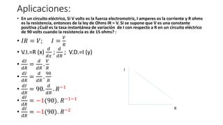
![Ejemplo
âĒ â ðĨ = ð[ð ðĨ ]ð
âĒ ââē(ðĨ) = ðâē ð ðĨ . ðâē(ðĨ)
âĒ â ðĨ =
4
(2ðĨ3 + 3ðĨ4 â ðĨ2)3
âĒ f ðĨ = 2ðĨ3 + 3ðĨ4 â ðĨ2 ; g x =
4
ðĨ3 = ðĨ
3
4
âĒ
âĒ ðâē ðĨ = 6ðĨ2 + 12ðĨ3 â 2ðĨ ; ðâē ðĨ =
3
44
ðĨ
âĒ ââē ðĨ =
3
4
4
2ðĨ3+3ðĨ4âðĨ2
. 6ðĨ2 + 12ðĨ3 â 2ðĨ
âĒ â ðĨ = ð ð ðĨ = (ððð)(ðĨ) Regla de la cadena
âĒ ââē(ðĨ) = ðâē ð ðĨ . ðâē(ðĨ)](https://image.slidesharecdn.com/derivacin1-211201152208/85/Derivacion-1-26-320.jpg)
![Ejemplo:
âĒ
ð
ððĨ
ðĢ. ðĒ =
ððĢ
ððĨ
. ðĒ +
ððĒ
ððĨ
. ðĢ
âĒ â ðĨ = ð ðĨ . [ð ðĨ ]
âĒ ââē ðĨ = ðâē ðĨ . ð ðĨ + [ðâē ðĨ . ð ðĨ ]
âĒ â ðĨ = [ ðĨ2 â 1 . ðĨ4 + ðĨ3 â 3ðĨ2 ]
âĒ ð ðĨ = ðĨ2 â 1 ð ðĨ = ðĨ4 + ðĨ3 â 3ðĨ2
âĒ ðâē ðĨ =
ð
ððĨ
ðĨ2 â
ð
ððĨ
1 ðâē ðĨ =
ð
ððĨ
ðĨ4 +
ð
ððĨ
ðĨ3 â 3.
ð
ððĨ
ðĨ2
âĒ ðâē ðĨ = 2x â 0 ðâē ðĨ = 4ðĨ3 + 3ðĨ2 â 6ðĨ
âĒ ââē ðĨ = 2x . ðĨ4 + ðĨ3 â 3ðĨ2 + [ 4ðĨ3 + 3ðĨ2 â 6ðĨ . ðĨ2 â 1 ]
âĒ ââē ðĨ = 2ðĨ5 + 2ðĨ4 â 6ðĨ3 + [4ðĨ5 + 3ðĨ4 â 6ðĨ3 â 4ðĨ3 â 3ðĨ2 + 6ðĨ]
âĒ ââē ðĨ = 2ðĨ5 + 2ðĨ4 â 6ðĨ3 + 4ðĨ5 + 3ðĨ4 â 6ðĨ3 â 4ðĨ3 â 3ðĨ2 + 6ðĨ
âĒ ââē ðĨ = 6ðĨ5 + 5ðĨ4 â 16ðĨ3 â 3ðĨ3 + 6ðĨ](https://image.slidesharecdn.com/derivacin1-211201152208/85/Derivacion-1-27-320.jpg)
![Ejemplo:
âĒ
ð
ððĨ
ðĢ/ðĒ =
[ ðĒ.
ððĢ
ððĨ
âðĢ.
ððĒ
ððĨ
]
ðĒ2
âĒ â ðĨ =
ð ðĨ
ð ðĨ
; ð ðĨ â 0
âĒ ââē ðĨ =
[ðâē ðĨ .ð ðĨ âðâē ðĨ .ð ðĨ ]
[ð(ðĨ)]2
âĒ â ðĨ = [
ðĨ2â1
ðĨ4+ðĨ3â3ðĨ2]
âĒ ð ðĨ = ðĨ2
â 1 ð ðĨ = ðĨ4
+ ðĨ3
â 3ðĨ2
âĒ ðâē
ðĨ =
ð
ððĨ
ðĨ2
â
ð
ððĨ
1 ðâē
ðĨ =
ð
ððĨ
ðĨ4
+
ð
ððĨ
ðĨ3
â 3.
ð
ððĨ
ðĨ2
âĒ ðâē ðĨ = 2x â 0 ðâē ðĨ = 4ðĨ3 + 3ðĨ2 â 6ðĨ
âĒ ââē
ðĨ =
[ 2x . ðĨ4+ðĨ3â3ðĨ2 â 4ðĨ3+3ðĨ2â6ðĨ .(ðĨ2â1)]
[ðĨ4+ðĨ3â3ðĨ2]2
âĒ ââē
ðĨ =
[ 2ðĨ5+2ðĨ4â6ðĨ3 â 4ðĨ5+3ðĨ4â6ðĨ3â4ðĨ3â3ðĨ2+6ðĨ ]
[ðĨ4+ðĨ3â3ðĨ2]2](https://image.slidesharecdn.com/derivacin1-211201152208/85/Derivacion-1-28-320.jpg)
![Ejemplo:
âĒ
ð
ððĨ
ðĢ/ðĒ =
[ ðĒ.
ððĢ
ððĨ
âðĢ.
ððĒ
ððĨ
]
ðĒ2
âĒ â ðĨ =
ð ðĨ
ð ðĨ
; ð ðĨ â 0
âĒ ââē ðĨ =
[ðâē ðĨ .ð ðĨ âðâē ðĨ .ð ðĨ ]
[ð(ðĨ)]2
âĒ ââē ðĨ =
[ 2ðĨ5+2ðĨ4â6ðĨ3 â 4ðĨ5+3ðĨ4â6ðĨ3â4ðĨ3â3ðĨ2+6ðĨ ]
[ðĨ4+ðĨ3â3ðĨ2]2
âĒ ââē ðĨ =
[2ðĨ5+2ðĨ4â6ðĨ3â4ðĨ5â3ðĨ4+6ðĨ3+4ðĨ3+3ðĨ2â6ðĨ]
[ðĨ4+ðĨ3â3ðĨ2]2
âĒ ââē
ðĨ =
[â2ðĨ5âðĨ4+4ðĨ3+3ðĨ2â6ðĨ]
[ðĨ4+ðĨ3â3ðĨ2]2](https://image.slidesharecdn.com/derivacin1-211201152208/85/Derivacion-1-29-320.jpg)
DerivaciÃģn 1.
- 1. DerivaciÃģn Ing. Mg. Luis Gabriel Lescano Paredes
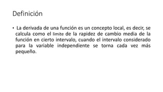
- 2. DefiniciÃģn âĒ La derivada de una funciÃģn es un concepto local, es decir, se calcula como el limite de la rapidez de cambio media de la funciÃģn en cierto intervalo, cuando el intervalo considerado para la variable independiente se torna cada vez mÃĄs pequeÃąo.
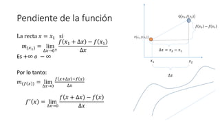
- 3. Pendiente de la funciÃģn La recta ðĨ = ðĨ1 si ð(ðĨ1) = lim âðĨâ0Âą ð ðĨ1 + âðĨ â ð ðĨ1 âðĨ Es +â ð â â Por lo tanto: ð(ð ðĨ ) = lim âðĨâ0 ð ðĨ+âðĨ âð ðĨ âðĨ ðâē ðĨ = lim âðĨâ0 ð ðĨ + âðĨ â ð ðĨ âðĨ P ð ðĨ1, ð ðĨ1 Q ðĨ2, ð ðĨ2 âðĨ = ðĨ2 â ðĨ1 ð ðĨ2 â ð ðĨ1 ðĨ2 ðĨ1 âðĨ
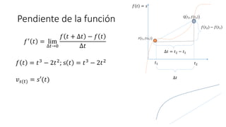
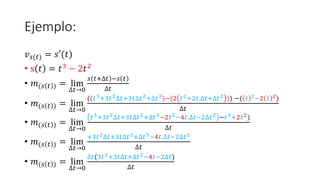
- 4. Pendiente de la funciÃģn ðâē ðĄ = lim âðĄâ0 ð ðĄ + âðĄ â ð ðĄ âðĄ ð ðĄ = ðĄ3 â 2ðĄ2; s ðĄ = ðĄ3 â 2ðĄ2 ðĢð (ðĄ) = ð âē(ðĄ) P ð ðĄ1, ð ðĄ1 Q ðĄ2, ð ðĄ2 âðĄ = ðĄ2 â ðĄ1 ð ðĄ2 â ð ðĄ1 ðĄ2 ðĄ1 âðĄ ð ðĄ = ð
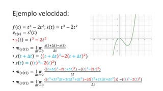
- 5. Ejemplo velocidad: ð ðĄ = ðĄ3 â 2ðĄ2; s ðĄ = ðĄ3 â 2ðĄ2 ðĢð (ðĄ) = ð âē(ðĄ) âĒ s ðĄ = ðĄ3 â 2ðĄ2 âĒ ð(ð ðĄ ) = lim âðĄâ0 ð ðĄ+âðĄ âð ðĄ âðĄ âĒ ð ðĄ + âðĄ = ( ðĄ + âðĄ 3â2 ðĄ + âðĄ 2) âĒ ð ðĄ = ( ðĄ 3â2 ðĄ 2) âĒ ð(ð ðĄ ) = lim âðĄâ0 ( ðĄ+âðĄ 3â2 ðĄ+âðĄ 2) â( ðĄ 3â2 ðĄ 2) âðĄ âĒ ð(ð ðĄ ) = lim âðĄâ0 ((ðĄ3+3ðĄ2âðĄ+3ðĄâðĄ2+âðĄ3)â(2 ðĄ2+2ðĄ.âðĄ+âðĄ2 )) â( ðĄ 3â2 ðĄ 2) âðĄ
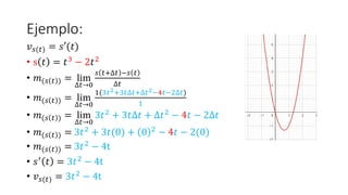
- 6. Ejemplo: ðĢð (ðĄ) = ð âē(ðĄ) âĒ s ðĄ = ðĄ3 â 2ðĄ2 âĒ ð(ð ðĄ ) = lim âðĄâ0 ð ðĄ+âðĄ âð ðĄ âðĄ âĒ ð(ð ðĄ ) = lim âðĄâ0 ((ðĄ3+3ðĄ2âðĄ+3ðĄâðĄ2+âðĄ3)â(2 ðĄ2+2ðĄ.âðĄ+âðĄ2 )) â( ðĄ 3â2 ðĄ 2) âðĄ âĒ ð(ð ðĄ ) = lim âðĄâ0 ðĄ3+3ðĄ2âðĄ+3ðĄâðĄ2+âðĄ3â2ðĄ2â4ðĄ.âðĄâ2âðĄ2 âðĄ3+2ðĄ2) âðĄ âĒ ð(ð ðĄ ) = lim âðĄâ0 +3ðĄ2âðĄ+3ðĄâðĄ2+âðĄ3â4ðĄ.âðĄâ2âðĄ2 âðĄ âĒ ð(ð ðĄ ) = lim âðĄâ0 âðĄ(3ðĄ2+3ðĄâðĄ+âðĄ2â4ðĄâ2âðĄ) âðĄ
- 7. Ejemplo: ðĢð (ðĄ) = ð âē(ðĄ) âĒ s ðĄ = ðĄ3 â 2ðĄ2 âĒ ð(ð ðĄ ) = lim âðĄâ0 ð ðĄ+âðĄ âð ðĄ âðĄ âĒ ð(ð ðĄ ) = lim âðĄâ0 1(3ðĄ2+3ðĄâðĄ+âðĄ2â4ðĄâ2âðĄ) 1 âĒ ð(ð ðĄ ) = lim âðĄâ0 3ðĄ2 + 3ðĄâðĄ + âðĄ2 â 4ðĄ â 2âðĄ âĒ ð(ð ðĄ ) = 3ðĄ2 + 3ðĄ(0) + 0 2 â 4ðĄ â 2(0) âĒ ð(ð ðĄ ) = 3ðĄ2 â 4t âĒ ð âē ðĄ = 3ðĄ2 â 4t âĒ ðĢð (ðĄ) = 3ðĄ2 â 4t
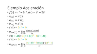
- 8. Ejemplo AceleraciÃģn âĒ ð ðĄ = ðĄ3 â 2ðĄ2 ; s ðĄ = ðĄ3 â 2ðĄ2 âĒ ðĢð (ðĄ) = ð âē(ðĄ) âĒ ðð (ðĄ) = ð âēâē(ðĄ) âĒ ðĢð (ðĄ) = ð âē(ðĄ) âĒ ð âē ðĄ = 3ðĄ2 â 4t âĒ ð(ð âē ðĄ ) = lim âðĄâ0 ð âē ðĄ+âðĄ âð âē ðĄ âðĄ âĒ ð âē ðĄ + âðĄ = 3(ðĄ + âðĄ)2 â4(ðĄ + âðĄ) âĒ ð âē ðĄ = 3ðĄ2 â 4t âĒ ð(ð âē ðĄ ) = lim âðĄâ0 (3 ðĄ+âðĄ 2â4 ðĄ+âðĄ )â(3ðĄ2â4t) âðĄ
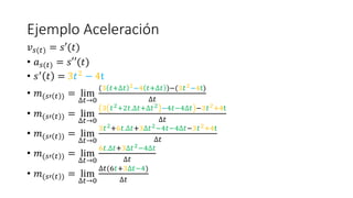
- 9. Ejemplo AceleraciÃģn ðĢð (ðĄ) = ð âē(ðĄ) âĒ ðð (ðĄ) = ð âēâē(ðĄ) âĒ ð âē ðĄ = 3ðĄ2 â 4t âĒ ð(ð âē ðĄ ) = lim âðĄâ0 (3 ðĄ+âðĄ 2â4 ðĄ+âðĄ )â(3ðĄ2â4t) âðĄ âĒ ð(ð âē ðĄ ) = lim âðĄâ0 3 ðĄ2+2ðĄ.âðĄ+âðĄ2 â4ðĄâ4âðĄ â3ðĄ2+4t âðĄ âĒ ð(ð âē ðĄ ) = lim âðĄâ0 3ðĄ2+6ðĄ.âðĄ+3âðĄ2â4ðĄâ4âðĄâ3ðĄ2+4t âðĄ âĒ ð(ð âē ðĄ ) = lim âðĄâ0 6ðĄ.âðĄ+3âðĄ2â4âðĄ âðĄ âĒ ð(ð âē ðĄ ) = lim âðĄâ0 âðĄ(6ðĄ+3âðĄâ4) âðĄ
- 10. Ejemplo AceleraciÃģn ðĢð (ðĄ) = ð âē(ðĄ) âĒ ðð (ðĄ) = ð âēâē(ðĄ) âĒ ð âē ðĄ = 3ðĄ2 â 4t âĒ ð(ð âē ðĄ ) = lim âðĄâ0 âðĄ(6ðĄ+3âðĄâ4) âðĄ âĒ ð(ð âē ðĄ ) = lim âðĄâ0 6ðĄ + 3âðĄ â 4 âĒ ð(ð âē ðĄ ) = 6ðĄ + 3(0) â 4 âĒ ð(ð âē ðĄ ) = 6ðĄ â 4 âĒ ð âēâē ðĄ = 6ðĄ â 4 âĒ ðð (ðĄ) = 6ðĄ â 4 âĒ ðð (ðĄ) = ðĢâēð (ðĄ)
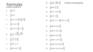
- 11. Formulas
- 12. Formulas
- 13. Formulas
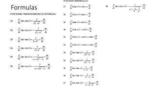
- 15. Formulas
- 16. Formulas
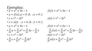
- 17. Ejemplos: âĒ ðĶ = ðĨ2 + 3ðĨ â 1 ð ðĨ = ðĨ2 + 3ðĨ â 1 âĒ ðĶ = ð ðĨ ;ðĶ = ð. ð·. ; ðĨ = ð. ðž. âĒ ð = ðĄ3 â 2ðĄ2 ð ðĄ = ðĄ3 â 2ðĄ2 âĒ ð = ð ðĄ ; ð = ð. ð·. ; ðĄ = ð. ðž. âĒ ðĶ = ðĨ2 + 3ðĨ â 1 ð ðĨ = ðĨ2 + 3ðĨ â 1 âĒ ð ððĨ ðĶ = ð ððĨ ðĨ2 + ð ððĨ 3ðĨ â ð ððĨ 1 ð ððĨ ð ðĨ = ð ððĨ ðĨ2 + ð ððĨ 3ðĨ â ð ððĨ 1 âĒ ð = ðĄ3 â 2ðĄ2 ð ðĄ = ðĄ3 â 2ðĄ2 âĒ ð ððĄ ð = ð ððĄ ðĄ3 â ð ððĄ 2ðĄ2 ð ððĄ ð ðĄ = ð ððĄ ðĄ3 â ð ððĄ 2ðĄ2
- 18. Ejemplos: âĒ ð ððĨ ð = 0 ; ðð ððĨ = 0; ðâē ð = 0 âĒ ðĶ = 5 ; ð§ = 3 ; ð ðĄ = 7 âĒ ð ððĨ ðĶ = ð ððĨ 5 ; ð ððĨ ð§ = ð ððĨ 3 ; ð ððĄ ð ðĄ = ð ððĄ 7 âĒ ððĶ ððĨ = 0 ; ðð§ ððĨ = 0 ; ðð(ðĄ) ððĄ = 0 ; fâē t = 0
- 19. Ejemplos: âĒ ð ððĨ ðĨ = 1 ; ððĨ ððĨ = 1 ; ð ðĨ = ðĨ âĒ ðâē ðĨ = 1 âĒ ðĶ = ðĨ + 1 ; ð§ = 3ðĨ â 2 ; ð ðĄ = 2ðĄ + 7 âĒ ð ððĨ ðĶ = ð ððĨ ðĨ + ð ððĨ 1 ; ð ððĨ ð§ = ð ððĨ 3ðĨ â ð ððĨ 2 ; ð ððĄ ð ðĄ = ð ððĄ 2ðĄ + ð ððĄ 7 âĒ ððĶ ððĨ = 1 + 0 ; ðð§ ððĨ = 3. ð ððĨ ðĨ â 0 ; ðâē ðĄ = 2. ð ððĄ ðĄ + 0 âĒ ððĶ ððĨ = 1 ; ðð§ ððĨ = 3. (1) ; ðâē ðĄ = 2. (1) âĒ ððĶ ððĨ = 1 ; ðð§ ððĨ = 3 ; ðâē ðĄ = 2
- 20. Ejemplo âĒ ð ððĨ ðĨ + ðĶ + ð§ = ð ððĨ ðĨ + ð ððĶ ðĶ + ð ðð§ ð§ âĒ ð ððĨ ð ðĨ + ð ðĨ + â ðĨ = ðâē ðĨ + ðâē ðĨ + ââē ðĨ âĒ ð ðĨ = 3ðĨ + 1 ; ð ðĨ = 9 ; â ðĨ = â2ðĨ âĒ ð ððĨ 3ðĨ + 1 + 9 + â2ðĨ = ð ððĨ ðĨ + 10 = ð ððĨ ðĨ + ð ððĨ 10 = 1 + 0 âĒ ð ððĨ 3ðĨ + 1 + 9 + â2ðĨ = 1
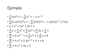
- 21. Ejemplo âĒ ð ððĨ ððĨð = ð. ð ððĨ ðĨð = ð. ð. ðĨðâ1 âĒ ð ððĨ ð. (ð ðĨ )ð = ð. ð ððĨ (ð ðĨ )ð= ð. ð. (ð ðĨ )ðâ1. ðâē(ðĨ) âĒ ðĶ = ðĨ4 + 2ðĨ2 + 3ðĨ + 1 âĒ ð ððĨ ðĶ = ð ððĨ ðĨ4 + ð ððĨ 2ðĨ2 + ð ððĨ 3ðĨ + ð ððĨ 1 âĒ ððĶ ððĨ = 4. ðĨ4â1 + 2. ð ððĨ ðĨ2 + 3. ð ððĨ ðĨ + 0 âĒ ððĶ ððĨ = 4. ðĨ3 + 2. 2ðĨ2â1 + 3. 1 + 0 âĒ ððĶ ððĨ = 4. ðĨ3 + 4ðĨ + 3
- 22. Ejemplo âĒ ð ððĨ ððĨð = ð. ð ððĨ ðĨð = ð. ð. ðĨðâ1 âĒ ð ððĨ ð. (ð ðĨ )ð = ð. ð ððĨ (ð ðĨ )ð = ð. ð. (ð ðĨ )ðâ1 . ðâē (ðĨ) âĒ ð ðĨ = 3 ðĨ3 â 2 ðĨ + 3ðĨâ2 + 5ðĨ1/7 âĒ ð ððĨ ð ðĨ = ð ððĨ 3 ðĨ3 â ð ððĨ 2 ðĨ + ð ððĨ 3ðĨâ2 + ð ððĨ 5ðĨ1/7 âĒ ðâē ðĨ = 3 ð ððĨ 1 ðĨ3 â 2 ð ððĨ ðĨ + 3 ð ððĨ ðĨâ2 + 5 ð ððĨ ðĨ1/7 âĒ ðâē ðĨ = 3 ð ððĨ ðĨâ3 â 2 ð ððĨ ðĨ 1 2 + 3 ð ððĨ ðĨâ2 + 5 ð ððĨ ðĨ 1 7 âĒ ðâē(ðĨ) = 3 â3 ðĨ(â3â1) â 2 ( 1 2 )ðĨ( 1 2 â1) + (3)(â2)ðĨ(â2â1) + (5)( 1 7 )ðĨ( 1 7 â1) âĒ ðâē ðĨ = â9ðĨ â4 â 1ðĨ â 1 2 â 6ðĨ(â3) + 5 7 ðĨ(â 6 7 ) âĒ ðâē ðĨ = â 9 ðĨ4 â 1 2 â 6 ðĨ3 + 5 7 7 ðĨ6
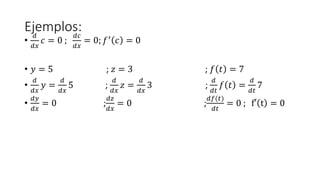
- 23. Ejemplo âĒ ð ððĨ ððĨð = ð. ð ððĨ ðĨð = ð. ð. ðĨðâ1 âĒ ð ððĨ ð. (ð ðĨ )ð = ð. ð ððĨ (ð ðĨ )ð= ð. ð. (ð ðĨ )ðâ1. ðâē(ðĨ) âĒ â ðĨ = 3(ð ðĨ )6 ; ð ðĨ = ðĨ3 + ðĨ2 + 1 âĒ ðâē ðĨ = 3ðĨ3â1 + 2ðĨ2â1 âĒ ðâē ðĨ = 3ðĨ2 + 2ðĨ âĒ ââē ðĨ = 3.6 ð ðĨ 6â1 . (ðâē ðĨ ) âĒ ââē ðĨ = 18 ðĨ3 + ðĨ2 + 1 5. (3ðĨ2 + 2ðĨ) âĒ â ðĨ = ð(ð ðĨ ); ð ðĨ = 3ðĨ6 ; ð ðĨ = ðĨ3 + ðĨ2 + 1 âĒ â ðĨ = 3(ðĨ3 + ðĨ2 + 1)6 âĒ ð ððĨ â ðĨ = ð ððĨ ((3(ðĨ3 + ðĨ2 + 1 )6))
- 24. Ejemplo âĒ ð ððĨ ð. (ð ðĨ )ð = ð. ð ððĨ (ð ðĨ )ð = ð. ð. (ð ðĨ )ðâ1 . ðâē (ðĨ) âĒ â ðĨ = ð(ð ðĨ ); ð ðĨ = 3ðĨ6 ; ð ðĨ = ðĨ3 + ðĨ2 + 1 âĒ ðâē ðĨ = 18ðĨ5 ; ð ðĨ = 3ðĨ2 + 2ðĨ âĒ â ðĨ = 3(ðĨ3 + ðĨ2 + 1)6 ; â ðĨ = ð(ð ðĨ )ð âĒ ââē ðĨ = c. ð. (ð ðĨ )ðâ1 . ðâē (ðĨ) âĒ â ðĨ = ð[ð ðĨ ]ð âĒ ââē ðĨ = ðâē ð ðĨ . ðâē (ðĨ) âĒ ð ððĨ â ðĨ = ð ððĨ ( 3 ðĨ3 + ðĨ2 + 1 6 ) âĒ ââē ðĨ = 3.6 ðĨ3 + ðĨ2 + 1 6â1. (3ðĨ2 + 2ðĨ) âĒ ââē ðĨ = 18 ðĨ3 + ðĨ2 + 1 5 . (3ðĨ2 + 2ðĨ)
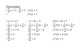
- 25. Ejemplo âĒ â ðĨ = ð[ð ðĨ ]ð âĒ ââē(ðĨ) = ðâē ð ðĨ . ðâē(ðĨ) âĒ â ðĨ = 4 (2ðĨ3 + 3ðĨ4 â ðĨ2)3 âĒ f ðĨ = 2ðĨ3 + 3ðĨ4 â ðĨ2 ; g x = 4 ðĨ3 = ðĨ 3 4 âĒ ðâē ðĨ = 6ðĨ2 + 12ðĨ3 â 2ðĨ ; ðâē ðĨ = 3 4 . ðĨ( 3 4 â1) âĒ ðâē ðĨ = 6ðĨ2 + 12ðĨ3 â 2ðĨ ; ðâē ðĨ = 3 4 . ðĨ(â 1 4 ) âĒ ðâē ðĨ = 3 4ðĨ 1 4 = 3 44 ðĨ
- 26. Ejemplo âĒ â ðĨ = ð[ð ðĨ ]ð âĒ ââē(ðĨ) = ðâē ð ðĨ . ðâē(ðĨ) âĒ â ðĨ = 4 (2ðĨ3 + 3ðĨ4 â ðĨ2)3 âĒ f ðĨ = 2ðĨ3 + 3ðĨ4 â ðĨ2 ; g x = 4 ðĨ3 = ðĨ 3 4 âĒ âĒ ðâē ðĨ = 6ðĨ2 + 12ðĨ3 â 2ðĨ ; ðâē ðĨ = 3 44 ðĨ âĒ ââē ðĨ = 3 4 4 2ðĨ3+3ðĨ4âðĨ2 . 6ðĨ2 + 12ðĨ3 â 2ðĨ âĒ â ðĨ = ð ð ðĨ = (ððð)(ðĨ) Regla de la cadena âĒ ââē(ðĨ) = ðâē ð ðĨ . ðâē(ðĨ)
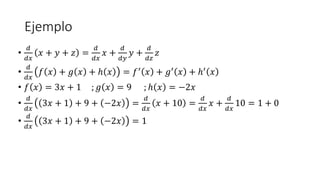
- 27. Ejemplo: âĒ ð ððĨ ðĢ. ðĒ = ððĢ ððĨ . ðĒ + ððĒ ððĨ . ðĢ âĒ â ðĨ = ð ðĨ . [ð ðĨ ] âĒ ââē ðĨ = ðâē ðĨ . ð ðĨ + [ðâē ðĨ . ð ðĨ ] âĒ â ðĨ = [ ðĨ2 â 1 . ðĨ4 + ðĨ3 â 3ðĨ2 ] âĒ ð ðĨ = ðĨ2 â 1 ð ðĨ = ðĨ4 + ðĨ3 â 3ðĨ2 âĒ ðâē ðĨ = ð ððĨ ðĨ2 â ð ððĨ 1 ðâē ðĨ = ð ððĨ ðĨ4 + ð ððĨ ðĨ3 â 3. ð ððĨ ðĨ2 âĒ ðâē ðĨ = 2x â 0 ðâē ðĨ = 4ðĨ3 + 3ðĨ2 â 6ðĨ âĒ ââē ðĨ = 2x . ðĨ4 + ðĨ3 â 3ðĨ2 + [ 4ðĨ3 + 3ðĨ2 â 6ðĨ . ðĨ2 â 1 ] âĒ ââē ðĨ = 2ðĨ5 + 2ðĨ4 â 6ðĨ3 + [4ðĨ5 + 3ðĨ4 â 6ðĨ3 â 4ðĨ3 â 3ðĨ2 + 6ðĨ] âĒ ââē ðĨ = 2ðĨ5 + 2ðĨ4 â 6ðĨ3 + 4ðĨ5 + 3ðĨ4 â 6ðĨ3 â 4ðĨ3 â 3ðĨ2 + 6ðĨ âĒ ââē ðĨ = 6ðĨ5 + 5ðĨ4 â 16ðĨ3 â 3ðĨ3 + 6ðĨ
- 28. Ejemplo: âĒ ð ððĨ ðĢ/ðĒ = [ ðĒ. ððĢ ððĨ âðĢ. ððĒ ððĨ ] ðĒ2 âĒ â ðĨ = ð ðĨ ð ðĨ ; ð ðĨ â 0 âĒ ââē ðĨ = [ðâē ðĨ .ð ðĨ âðâē ðĨ .ð ðĨ ] [ð(ðĨ)]2 âĒ â ðĨ = [ ðĨ2â1 ðĨ4+ðĨ3â3ðĨ2] âĒ ð ðĨ = ðĨ2 â 1 ð ðĨ = ðĨ4 + ðĨ3 â 3ðĨ2 âĒ ðâē ðĨ = ð ððĨ ðĨ2 â ð ððĨ 1 ðâē ðĨ = ð ððĨ ðĨ4 + ð ððĨ ðĨ3 â 3. ð ððĨ ðĨ2 âĒ ðâē ðĨ = 2x â 0 ðâē ðĨ = 4ðĨ3 + 3ðĨ2 â 6ðĨ âĒ ââē ðĨ = [ 2x . ðĨ4+ðĨ3â3ðĨ2 â 4ðĨ3+3ðĨ2â6ðĨ .(ðĨ2â1)] [ðĨ4+ðĨ3â3ðĨ2]2 âĒ ââē ðĨ = [ 2ðĨ5+2ðĨ4â6ðĨ3 â 4ðĨ5+3ðĨ4â6ðĨ3â4ðĨ3â3ðĨ2+6ðĨ ] [ðĨ4+ðĨ3â3ðĨ2]2
- 29. Ejemplo: âĒ ð ððĨ ðĢ/ðĒ = [ ðĒ. ððĢ ððĨ âðĢ. ððĒ ððĨ ] ðĒ2 âĒ â ðĨ = ð ðĨ ð ðĨ ; ð ðĨ â 0 âĒ ââē ðĨ = [ðâē ðĨ .ð ðĨ âðâē ðĨ .ð ðĨ ] [ð(ðĨ)]2 âĒ ââē ðĨ = [ 2ðĨ5+2ðĨ4â6ðĨ3 â 4ðĨ5+3ðĨ4â6ðĨ3â4ðĨ3â3ðĨ2+6ðĨ ] [ðĨ4+ðĨ3â3ðĨ2]2 âĒ ââē ðĨ = [2ðĨ5+2ðĨ4â6ðĨ3â4ðĨ5â3ðĨ4+6ðĨ3+4ðĨ3+3ðĨ2â6ðĨ] [ðĨ4+ðĨ3â3ðĨ2]2 âĒ ââē ðĨ = [â2ðĨ5âðĨ4+4ðĨ3+3ðĨ2â6ðĨ] [ðĨ4+ðĨ3â3ðĨ2]2
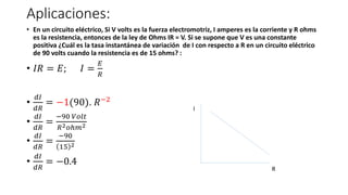
- 30. Aplicaciones: âĒ En un circuito elÃĐctrico, Si V volts es la fuerza electromotriz, I amperes es la corriente y R ohms es la resistencia, entonces de la ley de Ohms IR = V. Si se supone que V es una constante positiva ÂŋCuÃĄl es la tasa instantÃĄnea de variaciÃģn de I con respecto a R en un circuito elÃĐctrico de 90 volts cuando la resistencia es de 15 ohms? : âĒ ðžð = ð; ðž = ð ð âĒ V.I.=R (x) ð ððĨ ; ð ðð ; V.D.=I (y) âĒ ððž ðð = ð ðð . ð ð âĒ ððž ðð = ð ðð . 90 ð âĒ ððž ðð = 90. ð ðð . ð â1 âĒ ððž ðð = â1(90). ð â1â1 âĒ ððž ðð = â1(90). ð â2 I R
- 31. Aplicaciones: âĒ En un circuito elÃĐctrico, Si V volts es la fuerza electromotriz, I amperes es la corriente y R ohms es la resistencia, entonces de la ley de Ohms IR = V. Si se supone que V es una constante positiva ÂŋCuÃĄl es la tasa instantÃĄnea de variaciÃģn de I con respecto a R en un circuito elÃĐctrico de 90 volts cuando la resistencia es de 15 ohms? : âĒ ðžð = ðļ; ðž = ðļ ð âĒ ððž ðð = â1(90). ð â2 âĒ ððž ðð = â90 ððððĄ ð 2ðâð2 âĒ ððž ðð = â90 15 2 âĒ ððž ðð = â0.4 I R
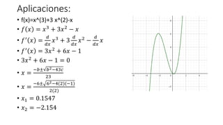
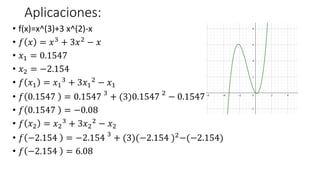
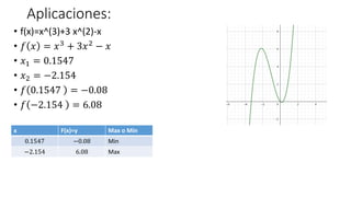
- 32. Aplicaciones: âĒ f(x)=x^(3)+3 x^(2)-x âĒ ð ðĨ = ðĨ3 + 3ðĨ2 â ðĨ âĒ ðâē ðĨ = ð ððĨ ðĨ3 + 3 ð ððĨ ðĨ2 â ð ððĨ ðĨ âĒ ðâē ðĨ = 3ðĨ2 + 6ðĨ â 1 âĒ 3ðĨ2 + 6ðĨ â 1 = 0 âĒ ðĨ = âðÂą ð2â43ð 23 âĒ ðĨ = â6Âą 62â4(2)(â1) 2(2) âĒ ðĨ1 = 0.1547 âĒ ðĨ2 = â2.154
- 33. Aplicaciones: âĒ f(x)=x^(3)+3 x^(2)-x âĒ ð ðĨ = ðĨ3 + 3ðĨ2 â ðĨ âĒ ðĨ1 = 0.1547 âĒ ðĨ2 = â2.154 âĒ ð ðĨ1 = ðĨ1 3 + 3ðĨ1 2 â ðĨ1 âĒ ð 0.1547 = 0.1547 3 + (3)0.1547 2 â 0.1547 âĒ ð 0.1547 = â0.08 âĒ ð ðĨ2 = ðĨ2 3 + 3ðĨ2 2 â ðĨ2 âĒ ð â2.154 = â2.154 3 + (3)(â2.154 )2 â(â2.154) âĒ ð â2.154 = 6.08
- 34. Aplicaciones: âĒ f(x)=x^(3)+3 x^(2)-x âĒ ð ðĨ = ðĨ3 + 3ðĨ2 â ðĨ âĒ ðĨ1 = 0.1547 âĒ ðĨ2 = â2.154 âĒ ð 0.1547 = â0.08 âĒ ð â2.154 = 6.08 x F(x)=y Max o Min 0.1547 â0.08 Min â2.154 6.08 Max
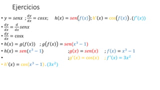
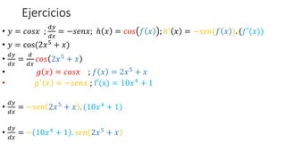
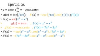
- 35. Ejercicios âĒ ðĶ = ð ðððĨ ; ððĶ ððĨ = ððð ðĨ; â ðĨ = ð ðð ð ðĨ ; ââē ðĨ = cos ð ðĨ . (ðâē(ðĨ)) âĒ ððĶ ððĨ = ð ððĨ ð ðððĨ âĒ ððĶ ððĨ = cosx âĒ â ðĨ = ð(ð ðĨ ) ; ð ð ðĨ = ð ðð(ðĨ3 â 1) âĒ â ðĨ = ð ðð(ðĨ3 â 1) ;ð ðĨ = ð ðð ðĨ ; ð ðĨ = ðĨ3 â 1 âĒ ;ðâē ðĨ = cos(ðĨ) ; ðâē ðĨ = 3ðĨ2 âĒ ââē ðĨ = cos ðĨ3 â 1 . (3ðĨ2)
- 36. Ejercicios âĒ ðĶ = ððð ðĨ ; ððĶ ððĨ = âð ðððĨ; â ðĨ = ððð ð ðĨ ; ââē ðĨ = âð ðð(ð ðĨ ). (ðâē(ðĨ)) âĒ ðĶ = cos(2ðĨ5 + ðĨ) âĒ ððĶ ððĨ = ð ððĨ ððð 2ðĨ5 + ðĨ âĒ ð ðĨ = ððð ðĨ ; ð ðĨ = 2ðĨ5 + ðĨ âĒ ðâē ðĨ = âð ðððĨ ; fâē(x) = 10ðĨ4 + 1 âĒ ððĶ ððĨ = âð ðð 2ðĨ5 + ðĨ . (10ðĨ4 + 1) âĒ ððĶ ððĨ = â 10ðĨ4 + 1 . ð ðð 2ðĨ5 + ðĨ
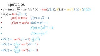
- 37. Ejercicios âĒ ðĶ = ðĄðððĨ ; ððĶ ððĨ = ð ðð2ðĨ; â ðĨ = ðĄðð ð ðĨ ; ââē ðĨ = ð ðð2(ð ðĨ ). (ðâē(ðĨ)) âĒ â ðĨ = tan ðĨ â 1 âĒ ð ðĨ = ðĄðððĨ ; ð ðĨ = ðĨ â 1 âĒ ðâē ðĨ = ð ðð2 ðĨ ; f ðĨ = ðĨ 1 2 â 1 âĒ ðâē(ðĨ) = 1 2 ðĨ 1 2 â1 â 0 âĒ ðâē(ðĨ) = 1 2 ðĨâ 1 2 âĒ ââē ðĨ = ð ðð2 ðĨ â 1 . ( 1 2 ðĨâ 1 2) âĒ ââē ðĨ = ( 1 2ðĨ 1 2 ). ð ðð2 ðĨ â 1 âĒ ââē ðĨ = ( 1 2 ðĨ ). ð ðð2 ðĨ â 1
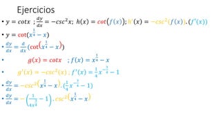
- 38. Ejercicios âĒ ðĶ = ðððĄðĨ ; ððĶ ððĨ = âðð ð2 ðĨ; â ðĨ = ðððĄ ð ðĨ ; ââē ðĨ = âðð ð2 (ð ðĨ ). (ðâē(ðĨ)) âĒ ðĶ = cot(ðĨ 1 4 â ðĨ) âĒ ððĶ ððĨ = ð ððĨ (cot ðĨ 1 4 â ðĨ ) âĒ ð ðĨ = ðððĄðĨ ; ð ðĨ = ðĨ 1 4 â ðĨ âĒ ðâē ðĨ = âðð ð2(ðĨ) ; ðâē ðĨ = 1 4 ðĨâ 3 4 â 1 âĒ ððĶ ððĨ = âðð ð2 ðĨ 1 4 â ðĨ . ( 1 4 ðĨâ 3 4 â 1) âĒ ððĶ ððĨ = â 1 4ðĨ 3 4 â 1 . ðð ð2 ðĨ 1 4 â ðĨ
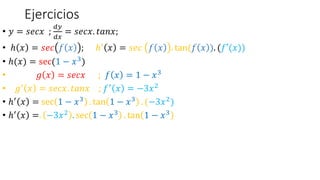
- 39. Ejercicios âĒ ðĶ = ð ðððĨ ; ððĶ ððĨ = ð ðððĨ. ðĄðððĨ; âĒ â ðĨ = ð ðð ð ðĨ ; ââē ðĨ = ð ðð ð ðĨ . tan(ð ðĨ ). (ðâē(ðĨ)) âĒ â(ðĨ) = sec(1 â ðĨ3) âĒ ð ðĨ = ð ðððĨ ; ð ðĨ = 1 â ðĨ3 âĒ ðâē ðĨ = ð ðððĨ. ðĄðððĨ ; ðâē ðĨ = â3ðĨ2 âĒ ââē ðĨ = sec 1 â ðĨ3 . tan 1 â ðĨ3 . (â3ðĨ2) âĒ ââē ðĨ =. â3ðĨ2 . sec 1 â ðĨ3 . tan 1 â ðĨ3
- 40. Ejercicios âĒ ðĶ = ðð ððĨ ; ððĶ ððĨ = âðð ððĨ. ðððĄðĨ; âĒ â ðĨ = ðð ð ð ðĨ ; ââē ðĨ = âðð ð ð ðĨ . ðððĄ(ð ðĨ ). (ðâē(ðĨ)) âĒ â(ðĨ) = csc(ðĨ7 â ðĨ3) âĒ ð ðĨ = ðð ððĨ ; ð ðĨ = ðĨ7 â ðĨ3 âĒ ðâē ðĨ = âðð ððĨ. ðððĄðĨ ; ðâē ðĨ = 7ðĨ6 â 3ðĨ2 âĒ ââē ðĨ = â csc ðĨ7 â ðĨ3 . cot ðĨ7 â ðĨ3 . (7ðĨ6 â 3ðĨ2) âĒ ââē ðĨ = â 7ðĨ6 â 3ðĨ2 . csc ðĨ7 â ðĨ3 . cot ðĨ7 â ðĨ3
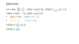
- 41. Ejercicios âĒ ðĶ = ðððĨ; ððĶ ððĨ = 1 ðĨ ; â ðĨ = ln(ð ðĨ ) ; ââē ðĨ = 1 ð ðĨ . (ðâē ðĨ ) âĒ â ðĨ = ln(ðĨ2 â 1) ; â ðĨ = ð(ð ðĨ ) âĒ ð ðĨ = ðððĨ ; ð ðĨ = ðĨ2 â 1 âĒ ðâē ðĨ = 1 ðĨ ; ðâē ðĨ = 2ðĨ âĒ ââē ðĨ = 1 ðĨ2â1 . (2ðĨ) âĒ ââē ðĨ = 2ðĨ ðĨ2â1
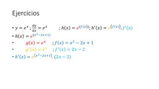
- 42. Ejercicios âĒ ðĶ = ððĨ ; ððĶ ððĨ = ððĨ ; â ðĨ = ð(ð(ðĨ)); ââē ðĨ = ð ð ðĨ . ðâē(ðĨ) âĒ â ðĨ = ð(ðĨ2â2ðĨ+1) âĒ ð ðĨ = ððĨ ; ð ðĨ = ðĨ2 â 2ðĨ + 1 âĒ ðâē ðĨ = ððĨ ; ðâē ðĨ = 2ðĨ â 2 âĒ ââē ðĨ = ð ðĨ2â2ðĨ+1 . (2ðĨ â 2)