�ݺ�ߣ

• Direct proportion is a type of proportionality relationship. For direct proportion, as
one value increases, so does the other value and conversely, as one value decreases,
so does the other value.
• The symbol ∝ represents a proportional relationship.
• If y is directly proportional to x, we can write this relationship as y x
∝
• Direct proportion is useful in numerous real-life situations, such as exchange rates,
unit conversion, and fuel prices.
Direct Proportion

If y is directly proportional to x, then y = k, where k is a
constant (number) called the constant of proportionality or
constant of variation.
A direct linear relationship exists between and y.
If increases (or decreases), y increases (or decreases)
If is doubled (or halved), y is doubled (or halved)
Another way of saying 'y is directly proportional to ' is y
varies directly with ‘
The graph of direct proportion is a straight line going
through (0, 0) with gradient k
Summary

The cost of a circular table is directly proportional to the square of the radius. " A circular table with a radius of
40cm cost $50.
" What is the cost of a circular table with a radius of 60cm? "
Problems

• Two variables are inversely proportional to each other if,
when one variable increases, the other one decreases by the
same factor.
• An example of inverse proportion would be the hours of
work required to build a wall. If there are more people
building the same wall, the time taken to build the wall
reduces.
Inverse Proportion

Inverse Proportion
If y is inversely proportional to x, then where k is a constant (number)
called the
constant of proportionality or constant of variation.
•If x increases, y decreases ('inverse' means 'opposite’)
•If x decreases, y increases
•If x is doubled, y is halved
•If x is halved, y is doubled
•Another way of saying 'y is inversely proportional to x' is 'y varies
inversely with

The time (t) in minutes taken by a car to travel 120 km is
inversely proportional to the speed (s in km/h) of the car. At
60 km/h, the time taken is 120 minutes.
a. Find the inverse variation equation for t.
b. How long did the car take to travel 120 km at:
i. 40 km/h?
ii. 110 km/h?
c. Find the car's speed if it took 45 minutes to travel 120 km.
Problems

The temperature, T (in degrees Celsius), of the air is inversely proportional to the
height, h (in meters), above sea level. At 800 m above sea level, the temperature is
10°C.
Questions:
a) What is the temperature at 1500 m above sea level?
b) Graph the relationship between temperature and height above sea level for
heights between 0 and 5000 m.
Problems

Two people take 15 minutes to clean the room. How many minutes will three people take to clean the same room?
Problems

Conversion graphs
Conversion graphs are straight line graphs that show a relationship between two
units and can be used to convert from one to another. They are very useful to solve
real-life problems.
Some conversion graphs can show a direct proportion between two units, for
example, converting between two currencies to show an exchange rate, such as
pounds sterling (British pounds) to US dollars.

1.Locate the values on the axis representing the
unit you wish to convert.
2.Draw a perpendicular line from the value on the
axis to the conversion line.
3.Draw a line from the conversion line
perpendicular to the other axis and read off the
conversion value.
How to use conversion graphs

different types of Graphs for Year10.pptx

Quadratic Function
• A function of the form y=ax2
+bx+c where a≠0
making a u-shaped graph called a parabola.
- If a is positive, u
opens up
- If a is negative, u
opens down
• The highest exponent of x is 2

𝑻𝒉𝒆𝒈𝒓𝒂𝒑𝒉𝒐𝒇 𝒚=𝒂𝒙𝟐
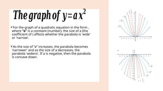
For the graph of a quadratic equation in the form ,
where “a” is a constant (number), the size of a (the
coefficient of ) affects whether the parabola is 'wide'
or 'narrow’.
As the size of “a” increases, the parabola becomes
'narrower' and as the size of a decreases, the
parabola 'widens'. If a is negative, then the parabola
is concave down.

+ C
•For the graph of a quadratic
equation in the form y = + c, where
a and c are constants, the effect of
c is to move the parabola up or
down from the origin. Also, c is the
y-intercept of the parabola.

Graph each set of quadratic Equations,
showing the vertex of each parabola
+5 ,

Graph each set of quadratic Equations,
showing the vertex of each parabola
,

Graphs of Exponential Functions

Note that in the definition of an exponential function, the base a = 1 is excluded
because it yields
f (x) = 1x
= 1.
This is a constant function, not an exponential function.
Exponential Functions

Real-life examples of exponential graph

Graphs of y = ax
In the same coordinate plane, sketch the graph of each function by
hand.
a. f(x) = 2x
b. g(x) = 4x
Solution:
The table below lists some values
for each function. By plotting these
points and connecting them with
smooth curves, you obtain the
graphs shown in Figure 3.1.
Figure 3.1

Note that both graphs are increasing. Moreover, the graph of
g(x) = 4x
is increasing more rapidly than the graph of
f(x) = 2x
. You can tell if you compare the y values in the table
below.
cont’d
Graphs of y = ax

Definition of a Circle
A circle is a set of points a given distance from one point
called the center.
The distance from the center is called the radius
Definition of a Circle

Find the equation of a circle with centre(0,0)
and diameter 25

�ݺ�ߣ

different types of Graphs for Year10.pptx

Recommended

More Related Content

Similar to different types of Graphs for Year10.pptx (20)

Recently uploaded (20)

different types of Graphs for Year10.pptx