DPB 10013 MICROECONOMICS (SUPPLY THEORY)
- 1. DPB 10013 : MICROECONOMICS CHAPTER 2 : SUPPLY
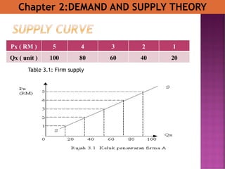
- 2. ’é× The ability and willingness to sell or produce a particular product and service in a given period of time at a particular price, Ceteris paribus . ’é× Supply schedule for a product is the list of quantity supplied at different prices assuming all other influences are constant. ’é× The table above shows the quantity supplied at each price level. Chapter 2:DEMAND AND SUPPLY THEORY
- 3. Px ( RM ) 5 4 3 2 1 Qx ( unit ) 100 80 60 40 20 Table 3.1: Firm supply Chapter 2:DEMAND AND SUPPLY THEORY
- 4. Px ( RM ) 5 4 3 2 1 Qx ( unit ) 100 80 60 40 20 Chapter 2:DEMAND AND SUPPLY THEORY
- 5. ’é× Individual supply ŌĆō the relationship between the quantity of a product supplied by a single seller and its price. ’é× Market supply ŌĆō the relationship between the total quantity of a product supplied by adding all the quantities supplied by all sellers in the market and its price. Chapter 2:DEMAND AND SUPPLY THEORY
- 6. Price X (RM ) Quantity of supply ( unit ) Market supply ( S )Firma A Firma B Firma C 5 12 16 20 48 4 9 12 18 39 3 7 9 16 32 2 5 6 14 25 1 0 2 12 14 Table 3.2: Market supply Chapter 2:DEMAND AND SUPPLY THEORY
- 7. Figure 3.2 : Supply curve firm A Chapter 2:DEMAND AND SUPPLY THEORY
- 8. Figure 3.3 : Supply curve firm B. Chapter 2:DEMAND AND SUPPLY THEORY
- 9. Figure 3.4 : Supply curve firm C. Chapter 2:DEMAND AND SUPPLY THEORY
- 10. Figure 3.5 : Market supply curve. Chapter 2:DEMAND AND SUPPLY THEORY
- 11. Law of supply ’é× The law of supply states that i. the higher the price of a product, the greater of the quantity supplied of that product and ii. the lower the price of a product, the lower of the quantity supplied, ceteris paribus. ’é× Positive relationship between price and quantity of supply ’é× Other factors is constant Supply function Qs = a + bP Chapter 2:DEMAND AND SUPPLY THEORY
- 12. ’é× Supply function ’é× Illustrates the relationship between quantity supply and price in a mathematical form. Qs =a + bP Where; Qs = the quantity of the supply goods(units) a = the quantity of the supply goods when the price (P) is zero. This value is intersect the quantity axis b = the gradient of the supply curve (a & b is variable) P = the price of the goods Chapter 2:DEMAND AND SUPPLY THEORY
- 13. Price (RM) 1 2 3 4 5 Quantity (Kg) 30 50 70 90 110 Table 3.3: Firm supply of shoes Chapter 2:DEMAND AND SUPPLY THEORY
- 14. Figure 3.6: Relationship between Price and Qs. Chapter 2:DEMAND AND SUPPLY THEORY
- 15. 1. Price of goods 2. Price of related goods (Substitute goods,complementary goods) 3. Level of technology 4. Production cost 5. Speculation 6. Government policies 7. Weather 8. Producer goals and expectations 9. Number of producer Chapter 2:DEMAND AND SUPPLY THEORY
- 16. ’é× Supply function Qs = a + bP ’é× Example 1: P 2 4 (i) 6( ii) 8 10 Qs 30 40 50 60 70 Table 3.3: supply of shoes Chapter 2:DEMAND AND SUPPLY THEORY
- 17. ’é× solution: Step 1: Qs = a + bP Step 2: i. 40 = a + 4b ii. 50 = a + 6b Equation (i) ŌĆō (ii) 40 - 50 = (a- a) + (4b ŌĆō 6b) -10 = -2b b = 10 / 2 b = 5 Chapter 2:DEMAND AND SUPPLY THEORY
- 18. ’é× Step 3: Sub b = 5 in equation (i) i. 40 = a + 4b 40 = a + 4 (5) 40 - 20 = a 20 = a Beside that; Qs = a + bP Qs = 20 + 5P# Chapter 2:DEMAND AND SUPPLY THEORY
- 19. ’é× Step 4: Check answer Qs = 20 + 5P# Equation (ii) ii. 50 = a + 5P 50 = 20 + 5(6) 50 = 20 + 30 50 = 50 Chapter 2:DEMAND AND SUPPLY THEORY
- 20. ’é× Example 2: ’é× Example 3: ’é× Example 4: P 2 4 6 8 10 Qs 20 40 60 80 100 P 1 2 3 4 Qs 20 24 28 32 P 1 2 3 4 Qs 24 26 28 30 Try your best!!! Chapter 2:DEMAND AND SUPPLY THEORY
- 21. ’é× To find the market supply curve, we need to calculate all the supply function of each firm ’é× Example 5: P Qs Ali Qs Abu Qs Amin Qs Market 1 0 10 50 60 2 (i) 5 20 100 125 3 (ii) 10 30 150 190 4 15 40 200 255 5 20 50 250 320 Table 3.3: Market supply of umbrella Chapter 2:DEMAND AND SUPPLY THEORY
- 22. ’é× Solution: Step 1: Qs = a + bP Step 2: ALI ABU AMIN i. 5 = a + 2b 20 = a + 2b 100 = a + 2b ii. 10 = a + 3b 30 = a + 3b 150 = a + 3b Equation (i) ŌĆō (ii) b = 5 b = 10 b = 50 Chapter 2:DEMAND AND SUPPLY THEORY
- 23. ’é× Step 3: Add b = in equation (i) 5 = a + 2b 20 = a + 2b 100 = a + 2b 5 = a + 2 (5) 20 = a + 2(10) 100 = a + 2(50) 5 = a + 10 20 - 20 = a 100 - 100 = a 5 - 10 = a a = -5 0 = a 0 = a So, the supply of firm market is; Qs = a + bP ALI ABU AMIN Qs = -5 + 5P Qs = 10P Qs = 50P Chapter 2:DEMAND AND SUPPLY THEORY
- 24. ’é× Qd Market = ALI = Qs = -5 + 5P ABU = Qs = 10P AMIN = Qs = 50P Qs = -5 + 65P Chapter 2:DEMAND AND SUPPLY THEORY
- 25. ’é× Example 6: P Qs Marsha Qs Milan Qs Londoh Qs Market 2 20 50 30 100 4 40 100 60 200 6 (i) 60 150 90 300 8 (ii) 80 200 120 400 10 100 250 150 500 Table 3.2: Market supply of handbag Chapter 2:DEMAND AND SUPPLY THEORY
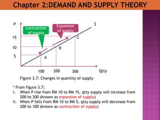
- 26. 1. Changes in quantity supply or movement along a supply curve - Occurs due to the price of the goods itself - When the price of the goods rises, the quantity supply will increase (known as expansion of supply) - When the price of the goods falls, the quantity supply will decrease (known as contraction of supply) Chapter 2:DEMAND AND SUPPLY THEORY
- 27. Chapter 2:DEMAND AND SUPPLY THEORY A C B SP Qtty 10 5 15 200100 300 Expansion of supply Contraction of supply Figure 3.7: Changes in quantity of supply * From figure 3.7; i. When P rise from RM 10 to RM 15, qtty supply will increase from 200 to 300 (known as expansion of supply) ii. When P falls from RM 10 to RM 5, qtty supply will decrease from 200 to 100 (known as contraction of supply)
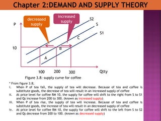
- 28. ii. Changes in supply or shift in supply curve - Occur when the supply curve shifts to the right or left due to changes in factors other than the price of the goods itself - The supply curve will shift to the left when the supply increases (known as increased supply) - The supply curve will shift to the left when the supply decreases (known as decreased supply). Chapter 2:DEMAND AND SUPPLY THEORY
- 29. Chapter 2:DEMAND AND SUPPLY THEORY A C B SP Qtty 10 200100 300 Figure 3.8: supply curve for coffee * From figure 3.8; i. When P of tea fall, the supply of tea will decrease. Because of tea and coffee is substitute goods, the decrease of tea will result in an increased supply of coffee ii. At price level for coffee RM 10, the supply for coffee will shift to the right from S to S1 and Qs increase from 200 to 300. (known as increased supply) iii. When P of tea rise, the supply of tea will increase. Because of tea and coffee is substitute goods, the increase of tea will result in an decreased supply of coffee iv. At price level for coffee RM 10, the supply for coffee will shift to the left from S to S2 and Qs decrease from 200 to 100. (known as decreased supply) S2 S1 decreased supply increased supply


