

![Industrial Economics EC4417
6
than the better it is as an estimateto explain the relationship between the variables or how
well the independent variables predict the explanatory variable. The purpose is for the
model to explain the variation in the dependent variable, in this case Market share. From
our results, we can see that RÂē=.9096 (appendix 1) which is quite high and suggests the
model is a good fit.
Significance of the Model:
We have used t-tests to test the significance of each individual independent variable and its
relationship with the dependent variable. As this is a multi-variable regression, however, the
f-test will provide us with a better overall assessment of models significance. The test can
also be seen as a test of the significance of RÂē and the value of that estimator.
The F-test is another form of hypothesis testing which we define as below:
ðŧ0: ðĩ1 = 0, ðĩ2 = 0 âĶ
ðŧ1: ðĩ1 ððððð ðĩ2 â 0
The formula to find the F-stat is as follows:
ðđ = (ð
2
/ðū)/[
1â ð
2
ð â ð â 1
]
The calculation shows Fstat=135.83628316 (appendix 2) and we now compare this to the
Fcrit value taken from the table of statistical distributions. Our degrees of freedom will read
as (2,27) and we will again take a 5% critical value. This gives an Fcrit=3.35, and we can see
that 135.83628>3.35 and therefore we can reject the null hypothesis and state that there is
a statistical significance in our models estimates.
Specification error test (Ramsey RESET test)
We have conducted Ramseyâs RESET test to check if we have omitted any significant
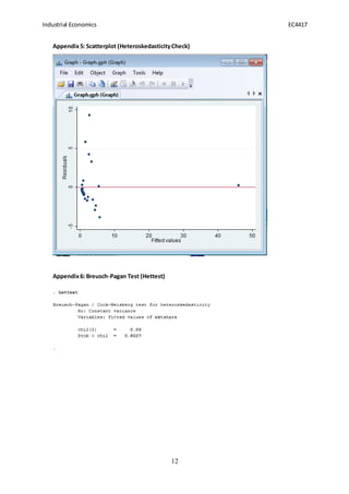
variables. To do this we created the new variable,yhatsq. We must present the null and
alternative hypothesis for the value of yhatsq once more:
ðŧ0: ðĩðĶâððĄð ð = 0
ðŧ1: ðĩðĶâððĄð ð â 0
If we reject the null hypothesis then we will conclude that we have omitted significant
variables. Choosing a 5% significance level, we compare the p-value for yhatsq as per the
RESET test (appendix 3) and find that .521>.05 and therefore accept the null and conclude
that we have not omitted significant variables from our model. We have included the
âovtestâ (appendix 4) we ran in Stata in our appendix which is consistent with these findings.
4.3 Violations of the assumptions of the Basic Regression Model
Heteroskedasticity:
The OLS model contains one assumption which assumes that the all variances of the random
error will remain constant, our in other words homoscedastic variances. A violation of this is
known as heteroskedasticity meaning we have differing variances in our data and that OLS
will no longer by the best linear estimator for our error.](https://image.slidesharecdn.com/f7735040-c002-4f6e-b8b9-7ce98e68bb32-150109131616-conversion-gate01/85/EC4417-Econometrics-Project-6-320.jpg)
![Industrial Economics EC4417
9
6. References
Ahearne,A.(2014) âThe economicrecovery is most visible in the labourmarketâ IrishTimes[online],
Aug9, available:http://www.irishtimes.com/business/economy/the-economic-recovery-is-most-
visible-in-the-labour-market-1.1891630?page=2 [accessed25 Nov2014]
Currim,I. S.,Lim,J. and JoungKim,W. (2012) âYou Get What You PayFor: The Effectof Top
ExecutivesâCompensationonAdvertisingandR&DSpendingDecisionsandStockMarketReturnâ,
Journalof Marketing [online],76(5),33-48, available:EBSCOBusinessSource Complete [accessed03
Dec 2014]
Enterprise Europe Network.(2012) Information,Communicationand Technology Sectorin Ireland
[online],available:http://www.een-
ireland.ie/eei/assets/documents/uploaded/general/ICT%20Fact%20sheet.pdf [accessed13 Nov
2014]
Grossmann,V.(2008) âAdvertising,In-House R&D,andGrowthâ, Oxford EconomicPapers [online],
60(1), 168-191, available:EconlitwithFullText[accessed26Nov2014]
SiliconRepublic(2013), Homegrown Irish tech sector thinksdifferently to overcometalent
bottleneck[online],available: http://www.siliconrepublic.com/careers/item/35189-homegrown-
irish-tech-sector[accessed13Nov2014]](https://image.slidesharecdn.com/f7735040-c002-4f6e-b8b9-7ce98e68bb32-150109131616-conversion-gate01/85/EC4417-Econometrics-Project-9-320.jpg)
![Industrial Economics EC4417
10
7. Appendix:
Appendix 1: FirstRegression
Appendix2: F-Test
ðđð ðĄððĄ = (ð
2
/ðū)/[
1 â ð
2
ð â ð â 1
]
ðđð ðĄððĄ = (
.9096
2
)/[
1 â .9096
30 â 2 â 1
]
ðđð ðĄððĄ = .4548/(
.0904
37
)
ðđð ðĄððĄ = 135.836283186
Appendix3: Ramsey RESET Test](https://image.slidesharecdn.com/f7735040-c002-4f6e-b8b9-7ce98e68bb32-150109131616-conversion-gate01/85/EC4417-Econometrics-Project-10-320.jpg)
EC4417 Econometrics Project
- 1. Industrial Economics EC4417 1 Department of Economics EC 4417 - Industrial Economics Project Autumn Semester 2014/15 Lecturer: Bernadette Andreosso-OâCallaghan Teaching Assistant: OlubunmiIpinnaiye Project Title: Relationship between Market Share, R&D expenditure and Advertising Group Members: Names ID Lonan O Cearbhaill 11135069 Gearoid Dowling 10080414 Brian Mullins 10116052 (To be completed by T.A.) Group Number:_______________
- 2. Industrial Economics EC4417 2 Contents 1. Introduction:........................................................................................................................ 3 2. Data: ....................................................................................................................................3 3. Methodology:....................................................................................................................... 4 4. Results:................................................................................................................................ 4 4.1 Report on the coefficients. ............................................................................................ 4 4.2 Measures of Fit............................................................................................................. 5 4.3 Violations of the assumptions of the Basic Regression Model:........................................6 5. Interpretation of Results and Conclusion:.............................................................................. 7 6. References:.............................................................................. Error! Bookmark not defined. 7. Appendix:.................................................................................................................... 10. /10
- 3. Industrial Economics EC4417 3 1. Introduction: The technology industry in Ireland is becoming increasingly important to contributing to growth in the Irish Economy. Med-tech and Information/Communications technology have been identified as key industries that are driving the Irish economic recovery (Ahearne 2014). Forty per cent of Irelandâs GDP (âŽ72bn) comes from its technology sector, which employs over 105,000 people. Since 2010, more than 18,000 jobs have been announced in the sector, making Ireland the go-to place to locate international tech headquarters. Ireland is one of the main locations worldwide where a career in IT can be advanced. Having said that our indigenous IT firms only account for âŽ2bn of that âŽ72bn but we make up 28.6% of the employment with 30,000 of the IT jobs (Silicon republic 2013). Key stats: ï· 9/10 global ICT companies maintain a presence in Ireland. ï· The top 5 software companies have a significant presence in Ireland. ï· The total number of ICT enterprises in Ireland is approximately 5,400; 233 of which are foreign owned. (Enterprise Europe Network 2012). The aim of this project is to construct a statistical model to assess the relationship between the dependent variable (Market share) and the two independent variables (advertising and R&D) within the technology industry. We will examine, through our statistical estimates, what companies and to a broader extent the government could learn from this report about how these variables interact in the technology sector and the implications it has on their decisions. Using the Ordinary Least Squares method, we will assess the relationship between the variables on the basis of the below model: Mkt Share= ð1 + ð2ð &ð· + ð3ðððĢ This will provide an estimate of the relationship between the variables which we expect to be positive. The reason for this is the presumption that an increase in R&D and/or advertising expenditure would also increase the % of Mkt Share a company holds in an industry. Volker Grossman carried out an empirical driven model to study the implications of R&D expenditure and advertising expenditure finding there to be a positive relationship between those two variables and the size of firms and we will use these findings as the basis for our models expected outcome (Grossman 2008). 2. Data: We are using data from the FAME databases to guide our model on the technology industry. We have chosen to use the % of market share held within each company when taking the total number of observations (30) as the entire industry. We have calculated this through taking a companyâs turnover/industry total turnover. This may be a limitation of the data as it is a small sample size within the entire industry but we believe
- 4. Industrial Economics EC4417 4 on the basis of comparison between the variablesâ relationship that it will give us readable results that would be a good estimate of the industry as a whole. Administration costs will be used to form the advertising variables as this information will contain the total spend and as Research and Development costs are specified we can use them directly in the model. It is also important to note that information regarding R&D expenditure is not readily available for Irish companies within the FAME database. We will therefore use UK companies in our model to form an understanding of the relationships between the variables in our model and explain what we can conclude from this with reference to the importance of the Technology industry within Ireland. 3. Methodology: OLS Method We will examine the relationships between the variables of our model by using regression analysis. For a population regression, we would assume the equation of a multi-variable regression to be as follows: ð = ðĩ1+ ðĩ2ðĨ + ðĩ3ðĨ + ð Of course the purpose of statistical analysis is to provide us with an estimate of the overall population as it is nearly impossible to accurately assess the population mean of the dependent variable with respect to available information. Instead, we use sample data where we say that ð1 and ð2 will be estimates of ðĩ1 and ðĩ2(the intercept and slope). Ordinary Least Squares (OLS) is the best linear estimate as it minimizes the squared error giving us a model that best fits the data we will use. To hold true, the OLS involves the following assumptions: ï· The regression should show the following relationship between the dependent variable (Y) for each independent variable (X): ð = ðĩ1 + ðĩ2ð + ð ï· The average value of the random error is: ðļ( ð) = 0 ï· That there is constant variance of the random error (Homoskedasticity): ðĢðð( ð) = ð2 = ðĢðð(ðĶ) ï· The covariance between any pair of errors is 0: ðķððĢ( ðð, ðð) = 0 4. Results: 4.1 Report on the coefficients. As we recall, we are testing our model using a sample regression for the population based on the below equation: Mkt Share= ð1 + ð2ð &ð· + ð3ðððĢ
- 5. Industrial Economics EC4417 5 We need to determine the coefficients for the parameters ð1 ððð ð2 in order to determine the slope of the line, which will tell us about the relationship between market share and the explanatory variables r&d and advertising. After running the regression (appendix 1), we can see that the coefficients are ð2ð&ð = .0306753and ð3ðððĢ = .0039812. The important thing to note here is the sign of the coefficients; they are both positive which suggests a positive relationship between dependent and explanatory variables meaning an increase in r&d and advertising expenditure is expected to lead to an increase in market share. When we look at the individual magnitude of the independent variables we can see in real terms how a unitincrease (taken as a %) affects the dependent variable. We can explain this more clearly that if R&D expenditure increases by 20% (20 units), then we can work out the increase in market share as 20 â 0.0306753 = .613506% increase in market share. Equally, we can apply the same formula to measure a 20% increase in advertising expenditure to increase market share as 20 â .0039812 = .079624%. We can deduce from these results that it takes quite a large increase in R&D and Advertising expenditure to make a significant increase in market share. The next step is to analyse the significance of each of the independent variables using hypothesis testing. We need to set up two hypotheses tests as follows: ðŧ0: ðĩ2 = 0, ðŧ1: ðĩ2 â 0 ðŧ0: ðĩ3 = 0, ðŧ1: ðĩ3 â 0 We know from economic theory that we need to use a T-test in order to accept/reject H0 (the null hypothesis). We calculated the degrees of freedom as df=N-K-1, or 30-1-1=28. Using a .05 significance level in a two-tailed test we found that ðððððĄ = 2.048. From our regression, we can see that for our R&D variable that ðð ðĄððĄ = 8.43. Our other variable, Advertising, shows a value ofðð ðĄððĄ = 1.81. This means we can reject the null hypothesis H0: B2=0 as 8.43>2.048. We cannot, however, reject the null hypothesis H0: B3=0 using a 95% confidence level given that 1.81<2.048. Further confirmation of this can be seen through our p-value, the exact level of significance. For our R&D variable, the p-value=0.00 which proves 0.05>0.00 meaning that there is a positive relationship between R&D expenditure and Market Share. The Advertising expenditure variable gives a p-value=0.082, which is 0.05<0.082 meaning it does not fall in the reject region and the null hypothesis is true at a 95% confidence level. In summary, we conclude that R&D variable is significant while our Advertising variable is not statistically significant. 4.2 Measures of fit: Fit: RÂē is known as the coefficient of determination and is the common estimate used to test the goodness of fit of our statistical model. The premise is that the closer to RÂē=1 the model is
- 6. Industrial Economics EC4417 6 than the better it is as an estimateto explain the relationship between the variables or how well the independent variables predict the explanatory variable. The purpose is for the model to explain the variation in the dependent variable, in this case Market share. From our results, we can see that RÂē=.9096 (appendix 1) which is quite high and suggests the model is a good fit. Significance of the Model: We have used t-tests to test the significance of each individual independent variable and its relationship with the dependent variable. As this is a multi-variable regression, however, the f-test will provide us with a better overall assessment of models significance. The test can also be seen as a test of the significance of RÂē and the value of that estimator. The F-test is another form of hypothesis testing which we define as below: ðŧ0: ðĩ1 = 0, ðĩ2 = 0 âĶ ðŧ1: ðĩ1 ððððð ðĩ2 â 0 The formula to find the F-stat is as follows: ðđ = (ð 2 /ðū)/[ 1â ð 2 ð â ð â 1 ] The calculation shows Fstat=135.83628316 (appendix 2) and we now compare this to the Fcrit value taken from the table of statistical distributions. Our degrees of freedom will read as (2,27) and we will again take a 5% critical value. This gives an Fcrit=3.35, and we can see that 135.83628>3.35 and therefore we can reject the null hypothesis and state that there is a statistical significance in our models estimates. Specification error test (Ramsey RESET test) We have conducted Ramseyâs RESET test to check if we have omitted any significant variables. To do this we created the new variable,yhatsq. We must present the null and alternative hypothesis for the value of yhatsq once more: ðŧ0: ðĩðĶâððĄð ð = 0 ðŧ1: ðĩðĶâððĄð ð â 0 If we reject the null hypothesis then we will conclude that we have omitted significant variables. Choosing a 5% significance level, we compare the p-value for yhatsq as per the RESET test (appendix 3) and find that .521>.05 and therefore accept the null and conclude that we have not omitted significant variables from our model. We have included the âovtestâ (appendix 4) we ran in Stata in our appendix which is consistent with these findings. 4.3 Violations of the assumptions of the Basic Regression Model Heteroskedasticity: The OLS model contains one assumption which assumes that the all variances of the random error will remain constant, our in other words homoscedastic variances. A violation of this is known as heteroskedasticity meaning we have differing variances in our data and that OLS will no longer by the best linear estimator for our error.
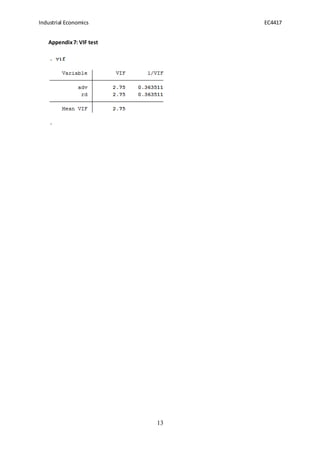
- 7. Industrial Economics EC4417 7 We can test for the variance using graphs to detect if there is a pattern in the change in variance. On our scatter plot (appendix 5) you can see that the value on the y axis quite high at beginning but curves towards the x-axis at the end. This seems to indicate the presence of heteroskedasticity, but we need to conduct a formal test in order to insure it is present in the model. The Breusch-Pagan test is the method we used in order to confirm our model was heteroskedastic. Once again we present the null and alternative hypotheses: ðŧ0: ðķððð ðĄðððĄ ðĢðððððððð ( ðŧðððð ððððð ðĄððððĄðĶ) ðŧ1: ð·ðððððððð ðĢðððððððð (ðŧððĄðððð ððððð ðĄððððĄðĶ) If the p-value of our chi square (prob>chi2) is smaller than the chosen level of significance (.05) then we would reject the null and conclude that there is heteroskedasticity in the model. The results of the Breusch-Pagan test (appendix 6) show p-value=.7812, .7812>.05 and therefore we cannot reject the Null and are satisfied that the assumption of constant variances hold and that we do not need to correct for heteroskedasticity as it is not present in our model. Multicollinearity: Multicollinearity is a feature of the sample and not the population and is therefore inevitably present in our model, thus the purpose of testing for it is to measure its degree. High multicollinearity can lead to large variances and covariances which in turn decreases the accuracy our estimation. It would mean ð 2 could be quite high despite one or more t ratios or the coefficients being statistically insignificant which would question if this measure of goodness of fit were actually accurate. One measure of detection for multicolinearity is if the RÂē is high but the individual t-tests of the variables suggest that none or very few are significant which would suggest it could be there to a large degree. In our model, RÂē=.9096 which is quite high but the advertising variable was statistically insignificant when we conducted the t-test. Formal testing of multicollinearity was required so we conducted the test for the Variance Inflation Factor (VIF) to measure the extent to which it is present in our model (appendix 7). VIF is measured as 1/Tolerance and we know that a VIF of over 10 would be a concern and merit further investigation to see if we could identify why it was so high in our model. The results show that for both the R&D and Advertising variable that VIF=2.75 which we deem to be low and thus are satisfied that we can conclude our investigation of mulitcollinearity. 5. Interpretation of Results and Conclusion: Our findings have shown that our model has yielded a good estimation of the relationship between the variables. The results indicate that there is a positive relationship between the dependent and independent variables and thus an increase in R&D expenditure and advertising will yield a greater % of market share for a company in the technology industry. We are happy that the model is a good fit, it is overall statistically significant and that we have not omitted any important variables. Our results
- 8. Industrial Economics EC4417 8 did show that advertising was not statistically significant and therefore would question its impact on % of Market share gained through a unit increase in this variable. We are also satisfied that there has been no great violation of the assumptions made in the OLS model and that it remains the appropriate and best linear estimate of our analysis between the variables relationship. Further study in this area is required, however, as our report is constrained by our data coming from UK companies and that information on R&D expenditure in particular is difficult to find for Irish companies. It is also important to note that the figures have been derived from the last available reports of each individual company which vary and are not necessarily up to date. The results have been in accordance with a study carried out to investigate the effect of Executivesâ Compensation on R&D expenditure, Advertising and Stock market return in which it was found that âadvertising and R&D spending is positively associated with stock market returnâ (Currim et al. 2012). The model has demonstrated that firms in the technology sector can benefit from greater investment in R&D and advertising. As was stated at the outset, the technology sector is becoming an increasingly important area for expanding growth in the Irish economy. The government could be informed by this to increase incentives in the form of tax allowances, grants etc. to promote greater investment in R&D in particular within these companies to help increase their competiveness and performance and promote further expansion in this industry.
- 9. Industrial Economics EC4417 9 6. References Ahearne,A.(2014) âThe economicrecovery is most visible in the labourmarketâ IrishTimes[online], Aug9, available:http://www.irishtimes.com/business/economy/the-economic-recovery-is-most- visible-in-the-labour-market-1.1891630?page=2 [accessed25 Nov2014] Currim,I. S.,Lim,J. and JoungKim,W. (2012) âYou Get What You PayFor: The Effectof Top ExecutivesâCompensationonAdvertisingandR&DSpendingDecisionsandStockMarketReturnâ, Journalof Marketing [online],76(5),33-48, available:EBSCOBusinessSource Complete [accessed03 Dec 2014] Enterprise Europe Network.(2012) Information,Communicationand Technology Sectorin Ireland [online],available:http://www.een- ireland.ie/eei/assets/documents/uploaded/general/ICT%20Fact%20sheet.pdf [accessed13 Nov 2014] Grossmann,V.(2008) âAdvertising,In-House R&D,andGrowthâ, Oxford EconomicPapers [online], 60(1), 168-191, available:EconlitwithFullText[accessed26Nov2014] SiliconRepublic(2013), Homegrown Irish tech sector thinksdifferently to overcometalent bottleneck[online],available: http://www.siliconrepublic.com/careers/item/35189-homegrown- irish-tech-sector[accessed13Nov2014]
- 10. Industrial Economics EC4417 10 7. Appendix: Appendix 1: FirstRegression Appendix2: F-Test ðđð ðĄððĄ = (ð 2 /ðū)/[ 1 â ð 2 ð â ð â 1 ] ðđð ðĄððĄ = ( .9096 2 )/[ 1 â .9096 30 â 2 â 1 ] ðđð ðĄððĄ = .4548/( .0904 37 ) ðđð ðĄððĄ = 135.836283186 Appendix3: Ramsey RESET Test
- 11. Industrial Economics EC4417 11 Appendix4: Ovtest
- 12. Industrial Economics EC4417 12 Appendix5: Scatterplot (HeteroskedasticityCheck) Appendix6: Breusch-Pagan Test (Hettest)
- 13. Industrial Economics EC4417 13 Appendix7: VIF test