


Eigenstates of 2D Random Walk with Multiple Absorbing States
- 1. RANDOMWALKS, ABSORBING STATES, ANDYOU Kyle Poe | MATH 145 | February 27, 2018
- 2. APPLICATIONS OF RANDOM WALKS ŌĆó A random walk describes a stochastic process which takes a state into a series of consecutive following states which cannot be predetermined. ŌĆó Analysis of random walks can give us insight into important questions like: ŌĆó Will a drunk find his way home? ŌĆó Will a bee escape a trap? ŌĆó How will a gas diffuse?
- 3. ŌĆ£Given two states from which a stochastic 2-D system cannot escape, what is the probability of ending in either given some starting configuration?ŌĆØ
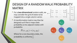
- 4. DESIGN OF A RANDOMWALK PROBABILITY MATRIX ŌĆó For a two-dimensional random walk, we may consider the grid of states to be mapped into a single column vector. ŌĆó A transformation matrix may then be designed such that it maps state probability z into adjacent states with probability Where for a non-boundary state, the probability is uniformly 1 5 . px,y px,y+1 px+1,y px,y-1 px-1,y
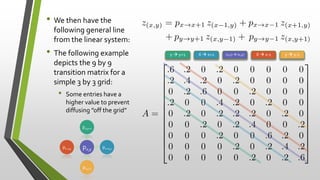
- 5. ŌĆó We then have the following general line from the linear system: ŌĆó The following example depicts the 9 by 9 transition matrix for a simple 3 by 3 grid: ŌĆó Some entries have a higher value to prevent diffusing ŌĆØoff the gridŌĆØ y ’āĀ y+1 X ’āĀ x+1 (x,y) ’āĀ (x,y) X ’āĀ x-1 y ’āĀ y-1 px,y px,y+1 px+1,y px,y-1 px-1,y
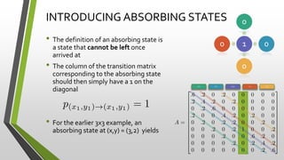
- 6. y+1 x+1 (x,y) x-1 y-1 INTRODUCING ABSORBING STATES ŌĆó The definition of an absorbing state is a state that cannot be left once arrived at ŌĆó The column of the transition matrix corresponding to the absorbing state should then simply have a 1 on the diagonal ŌĆó For the earlier 3x3 example, an absorbing state at (x,y) = (3,2) yields 1 0 0 0 0
- 7. SPECTRAL DECOMPOSITION ŌĆó By design, the matrix has stable eigenvectors corresponding to the ŌĆØsinkŌĆØ states ŌĆó For holes at (3,2), and (3,3), we have the following visualization of the stable eigenvectors: ŌĆó As can be seen in the next slide, all other eigenvectors have eigenvalues less than 1, so all steady states must therefore be superpositions of these two states ØæŻ1 = ØæŻ2 =
- 8. LONGTERM BEHAVIOR ŌĆó We will now direct our attention to a 75 by 75 version of the system with sinks at (10,10) and (20,20) (much more exciting!) ŌĆó Given our knowledge of the behavior of diagonal matrices, the following leads us back to our earlier conclusion that the final state is a superposition of the sinks: ŌĆó This assertion is further supported graphically!
- 9. LONGTERM BEHAVIOR -VISUALIZED ŌĆó Although the scope of time is too large to observe in a tolerable animation, there is indeed convergence to the distribution predicted by the method outlined on the previous slide. ŌĆó This kind of analysis can be performed on ANY random walk scenario, including those which have non-equal diffusing possibility