Excel Conditional Formatting
- 1. Excel Conditional Formatting Use Excel conditional formatting to set rules for cell formatting based on cell value or another cell.
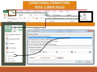
- 2. CONDITIONAL FORMATTING PATH -1 (NEW RULE)
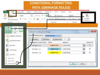
- 3. CONDITIONAL FORMATTING PATH -2(MANAGE RULES)
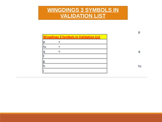
- 4. WINGDINGS 3 SYMBOLS IN VALIDATION LIST p Wingdings 3 Symbols in Validation List p > tu = q < q f g h tu i
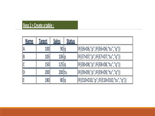
- 5. Step1>Createatable: Name Target Sales Status A 100 90 q IF(E6>D6,"p",IF(E6=D6,"tu","q")) B 105 106 p IF(E7>D7,"p",IF(E7=D7,"tu","q")) C 150 125 q IF(E8>D8,"p",IF(E8=D8,"tu","q")) D 200 200 tu IF(E9>D9,"p",IF(E9=D9,"tu","q")) E 180 80 q IF(E10>D10,"p",IF(E10=D10,"tu","q"))
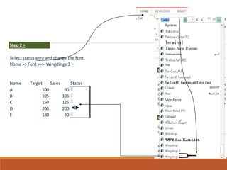
- 6. Step 2 > Select status area and change the font. Home >> Font >>> Wingdings 3 Name Target Sales Status A 100 90 q B 105 106 q C 150 125 q D 200 200 tu E 180 80 q
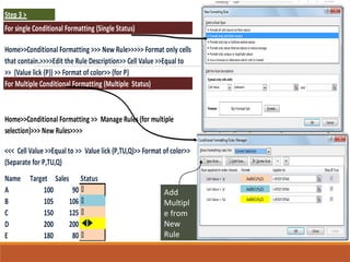
- 7. Add Multipl e from New Rule Step 3 > For single Conditional Formatting (Single Status) For Multiple Conditional Formatting (Multiple Status) Name Target Sales Status A 100 90 q B 105 106 q C 150 125 q D 200 200 tu E 180 80 q Home>>Conditional Formatting >>> New Rule>>>>> Format only cells that contain.>>>>Edit the Rule Description>> Cell Value >>Equal to >> (Value lick (P)) >> Format of color>> (for P) Home>>Conditional Formatting >> Manage Rules (for multiple selection)>>> New Rules>>>> <<< Cell Value >>Equal to >> Value lick (P,TU,Q)>> Format of color>> (Separate for P,TU,Q)
- 8. ?
- 9. Thanks You… Parveen Kumar Sharma. parveengarh@yahoo.com 9818580648
- 10. Thanks You… Parveen Kumar Sharma. parveengarh@yahoo.com 9818580648

