


More Related Content
What's hot (12)
Explicitarea recurentelor fundamentale s.boga
- 1. EXPLICITAREA RECUREN╚ÜELOR FUNDAMENTALE Tutorial redactat de Silviu Boga, mail: silviumath@yahoo.com Cuprins: ’éĘ Recuren┼Ża telescopic─ā aditiv─ā ’éĘ Progresiile aritmetice ’éĘ Recuren┼Ża telescopic─ā multiplicativ─ā ’éĘ Progresiile geometrice ’éĘ Recuren┼Ża liniar─ā neomogen─ā de ordin I, cu coeficien┼Żi variabili ’éĘ Recuren┼Ża liniar─ā neomogen─ā de ordin I, cu coeficien┼Żi constan┼Żi ’éĘ Recuren┼Ża liniar─ā omogen─ā de ordin II, cu coeficien┼Żi variabili ’éĘ Recuren┼Ża liniar─ā omogen─ā de ordin II, cu coeficien┼Żi constan┼Żi ’éĘ Recuren┼Ża liniar─ā neomogen─ā de ordin II, cu coeficien┼Żi constan┼Żi ’éĘ Recuren┼Że liniare omogene de ordin superior, cu coeficien┼Żi constan┼Żi ’éĘ Recuren┼Że liniare neomogene de ordin superior, cu coeficien┼Żi constan┼Żi ’éĘ Recuren┼Ża omografic─ā, cu coeficien┼Żi variabili ’éĘ Recuren┼Ża omografic─ā, cu coeficien┼Żi constan┼Żi Not─ā: - click pe titlul din cuprins pentru hyperlink spre fiecare recuren╚ø─ā - click pe num─ārul paginii pentru a reveni la cuprins
- 2. EXPLICITAREA RECUREN┼óELELOR FUNDAMENTALE La fiecare din recuren┼Żele urm─ātoare - fundamentale datorit─ā prezen┼Żei lor ├«n numeroase ra┼Żionamente matematice ŌĆō am prezentat, pe cazul general dar ┼¤i pe un exemplu, procedura optim─ā de explicitare. Prin rezolvarea temei de aprofundare, cititorul interesat se va putea apoi rapid acomoda cu judec─ā┼Żile expuse. 1. Recuren┼Ża telescopic─ā aditiv─ā ’ā¼ xn ’Ć½1 ’ĆĮ xn ’Ć½ an , (’Ćó)n ’āÄ * ’ā» ’āŁ x1 ’ĆĮ termen ini┼Żial dat ’ā»(a ) ’ĆŁ ┼¤ir explicit dat ’ā« n n’āÄ * Explicitare Din rela┼Żia de recuren┼Ż─ā, cum xn’Ć½1 ’ĆŁ xn ’ĆĮ an , (’Ćó)n ’āÄ * , prin particularizare ┼¤i sumare are loc supranumita reducere telescopic─ā ┼¤i explicitarea este astfel finalizat─ā: x2 ’ĆŁ x1 ’ĆĮ a1 x3 ’ĆŁ x2 ’ĆĮ a2 x4 ’ĆŁ x3 ’ĆĮ a3 ŌĆ”ŌĆ”ŌĆ”ŌĆ”ŌĆ”ŌĆ” xn ’ĆŁ1 ’ĆŁ xn ’ĆŁ2 ’ĆĮ an ’ĆŁ2 xn ’ĆŁ xn ’ĆŁ1 ’ĆĮ an ’ĆŁ1 ____________ (’Ć½) n ’ĆŁ1 n ’ĆŁ1 ’ā× xn ’ĆŁ x1 ’ĆĮ ’āź ak ’ā× xn ’ĆĮ x1 ’Ć½ ’āź ak k ’ĆĮ1 k ’ĆĮ1 n ’ĆŁ1 ├Än aplica┼Żiile curente suma iterat─ā ’āźa k ’ĆĮ1 k se va constata de regul─ā calculabil─ā. Se re┼Żin formulele de calcul pentru principalele sume iterate, ele fiind deosebit de utile ├«n procesele de explicitare ce vor urma: n n(n ’Ć½ 1) ’ü│ 1 ’ĆĮ ’āź k ’ĆĮ 1 ’Ć½ 2 ’Ć½ 3 ’Ć½ ... ’Ć½ n ’ĆĮ (I) k ’ĆĮ1 2 n n(n ’Ć½ 1)(2n ’Ć½ 1) ’ü│ 2 ’ĆĮ ’āź k 2 ’ĆĮ 12 ’Ć½ 22 ’Ć½ 32 ’Ć½ ... ’Ć½ n 2 ’ĆĮ (II) k ’ĆĮ1 6 ’ā® n(n ’Ć½ 1) ’ā╣ 2 n ’ü│ 3 ’ĆĮ ’āź k ’ĆĮ 1 ’Ć½ 2 ’Ć½ 3 ’Ć½ ... ’Ć½ n ’ĆĮ ’ā¬ 3 3 3 3 3 (III) k ’ĆĮ1 ’ā½ 2 ’ā║ ’ā╗ n an ’Ć½1 ’ĆŁ 1 ’ü░ ’ĆĮ ’āź a ’ĆĮ 1 ’Ć½ a ’Ć½ a ’Ć½ ... ’Ć½ a ’ĆĮ k 2 n (IV) k ’ĆĮ0 a ’ĆŁ1 ŌĆō1ŌĆō
- 3. La fel de util─ā se va dovedi ├«n acest sens ┼¤i procedura de descompunere a frac┼Żiilor ra┼Żionale ├«n supranumitele sume de frac┼Żii simple (metoda coeficien┼Żilor n nedetermina┼Żi), care va facilita calculul unor sume iterate ’āźt k ’ĆĮ1 k cu termenul general, f (k ) tk ’ĆĮ , frac┼Żii av├ónd f (k ) ┼¤i g (k ) expresii polinomiale. g (k ) n Din aceast─ā categorie de sume cel mai simplu de calculat sunt ’āźt k ’ĆĮ1 k cu 1 tk ’ĆĮ . ├Än astfel de cazuri se va observa cu u┼¤urin┼Ż─ā c─ā identificarea (ak ’Ć½ b)(ak ’Ć½ a ’Ć½ b) 1 A B ’ĆĮ ’Ć½ conduce la descompunerea termenului (ak ’Ć½ b)(ak ’Ć½ a ’Ć½ b) ak ’Ć½ b ak ’Ć½ a ’Ć½ b 1 1’ā” 1 1 ’āČ general sub forma ’ĆĮ ’ā¦ ’ĆŁ ’āĘ. (ak ’Ć½ b)(ak ’Ć½ a ’Ć½ b) a ’ā© ak ’Ć½ b ak ’Ć½ a ’Ć½ b ’āĖ De remarcat c─ā aici descompunerea poate chiar ocoli metoda coeficien┼Żilor 1 1 a nedetermina┼Żi, observ├ónd pur ┼¤i simplu ’ĆŁ ’ĆĮ , ak ’Ć½ b ak ’Ć½ a ’Ć½ b (ak ’Ć½ b )(ak ’Ć½ a ’Ć½ b ) 1 1’ā” 1 1 ’āČ deci tk ’ĆĮ ’ĆĮ ’ā¦ ’ĆŁ ’āĘ. (ak ’Ć½ b)(ak ’Ć½ a ’Ć½ b) a ’ā© ak ’Ć½ b ak ’Ć½ a ’Ć½ b ’āĖ Aceast─ā exprimare a termenului general t k , aplicat─ā succesiv, va pune ├«n eviden┼Ż─ā cunoscuta reducere telescopic─ā prin care de altfel se va ┼¤i finaliza calculul sumei, dup─ā cum ilustreaz─ā ┼¤i urm─ātorul exemplu: 1 1 1 1 Sn ’ĆĮ ’Ć½ ’Ć½ ’Ć½ ... ’Ć½ 7 ’āŚ 11 11’āŚ 15 15 ’āŚ 19 (4n ’Ć½ 3) ’āŚ (4n ’Ć½ 7) 1 Solu┼Żie Se observ─ā termen general tk ’ĆĮ , k ’āÄ 1 n , apoi ; (4k ’Ć½ 3)(4k ’Ć½ 7) 1 1 4 1 1’ā” 1 1 ’āČ ’ĆŁ ’ĆĮ ’ā× tk ’ĆĮ ’ĆĮ ’ā¦ ’ĆŁ ’āĘ din 4k ’Ć½ 3 4k ’Ć½ 7 (4k ’Ć½ 3)(4k ’Ć½ 7) (4k ’Ć½ 3)(4k ’Ć½ 7) 4 ’ā© 4k ’Ć½ 3 4k ’Ć½ 7 ’āĖ care, prin particularizare ┼¤i sumare, apare reducerea telescopic─ā ce finalizeaz─ā calculul, 1 1’ā” 1 1 ’āČ t1 ’ĆĮ ’ĆĮ ’ā¦ ’ĆŁ ’āĘ 7 ’āŚ 11 4 ’ā© 7 11 ’āĖ 1 1’ā” 1 1’āČ t2 ’ĆĮ ’ĆĮ ’ā¦ ’ĆŁ ’āĘ 11’āŚ 15 4 ’ā© 11 15 ’āĖ ŌĆ”ŌĆ”ŌĆ”ŌĆ”ŌĆ”ŌĆ”ŌĆ”ŌĆ”ŌĆ”ŌĆ”ŌĆ”ŌĆ”ŌĆ”ŌĆ”ŌĆ”ŌĆ”ŌĆ”ŌĆ”.. 1 1’ā” 1 1 ’āČ tn ’ĆĮ ’ĆĮ ’ā¦ ’ĆŁ ’āĘ, (4n ’Ć½ 3) ’āŚ (4n ’Ć½ 7) 4 ’ā© 4n ’Ć½ 3 4n ’Ć½ 7 ’āĖ ŌĆō2ŌĆō
- 4. ob┼Żin├óndu-se la final n 1 ’ā®’ā” 1 1 ’āČ ’ā” 1 1 ’āČ ’ā” 1 1 ’āČ’ā╣ 1 ’ā” 1 1 ’āČ n Sn ’ĆĮ ’āź t k ’ĆĮ ’ā¬’ā¦ ’ĆŁ ’āĘ ’Ć½ ’ā¦ ’ĆŁ ’āĘ ’Ć½ ... ’Ć½ ’ā¦ ’ĆŁ ’āĘ’ā║ ’ĆĮ ’ā¦ ’ĆŁ ’āĘ’ĆĮ k ’ĆĮ1 4 ’ā½’ā© 7 11’āĖ ’ā© 11 15 ’āĖ ’ā© 4n ’Ć½ 3 4n ’Ć½ 7 ’āĖ ’ā╗ 4 ’ā© 7 4n ’Ć½ 7 ’āĖ 7(4n ’Ć½ 7) Acestea fiind prezentate, revin la recuren┼Ża telescopic─ā aditiv─ā, cu parcurgerea algoritmului de explicitare pe un caz concret. ’ā¼ x ’ĆĮ xn ’Ć½ n(n ’Ć½ 1), (’Ćó)n ’āÄ * Exemplu Explicitez ┼¤irul generat de recuren┼Ża ’āŁ n ’Ć½1 ’ā« x1 ’ĆĮ 1 Solu┼Żie xn’Ć½1 ’ĆŁ xn ’ĆĮ n(n ’Ć½ 1), (’Ćó)n ’āÄ * ┼¤i astfel x2 ’ĆŁ x1 ’ĆĮ 1’āŚ 2 x3 ’ĆŁ x 2 ’ĆĮ 2 ’āŚ 3 x 4 ’ĆŁ x3 ’ĆĮ 3 ’āŚ 4 ŌĆ”ŌĆ”ŌĆ”ŌĆ”ŌĆ”ŌĆ” xn ’ĆŁ1 ’ĆŁ xn ’ĆŁ2 ’ĆĮ (n ’ĆŁ 2) ’āŚ (n ’ĆŁ 1) xn ’ĆŁ xn ’ĆŁ1 ’ĆĮ (n ’ĆŁ 1) ’āŚ n ____________ (’Ć½) n ’ĆŁ1 n ’ĆŁ1 ’ā× xn ’ĆŁ x1 ’ĆĮ ’āź k (k ’Ć½ 1) ┼¤i cum x1 ’ĆĮ 1 ’ā× xn ’ĆĮ 1 ’Ć½ ’āź k (k ’Ć½ 1) , sum─ā care este k ’ĆĮ1 k ’ĆĮ1 u┼¤or calculabil─ā cu ajutorul formulelor sumelor remarcabile anterior prezentate, n ’ĆŁ1 n ’ĆŁ1 n ’ĆŁ1 (n ’ĆŁ 1)n(2n ’ĆŁ 1) (n ’ĆŁ 1)n respectiv xn ’ĆĮ 1 ’Ć½ ’āź k (k ’Ć½ 1) ’ĆĮ 1 ’Ć½ ’āź k 2 ’Ć½ ’āź k ’ĆĮ 1 ’Ć½ ’Ć½ , etc. k ’ĆĮ1 k ’ĆĮ1 k ’ĆĮ1 6 2 Tem─ā de aprofundare Proced├ónd analog, explicita┼Żi urm─ātoarele recuren┼Że: ’ā¼ x ’ĆĮ xn ’Ć½ (2n ’Ć½ 1), (’Ćó)n ’āÄ * ’ā¼ x ’ĆĮ xn ’Ć½ n(n ’Ć½ 1)(2n ’Ć½ 1), (’Ćó)n ’āÄ * a) ’āŁ n ’Ć½1 b) ’āŁ n ’Ć½1 ’ā« x1 ’ĆĮ 1 ’ā« x1 ’ĆĮ 1 ’ā¼ 1 ’ā¼ 1 ’ā» xn ’Ć½1 ’ĆĮ xn ’Ć½ , (’Ćó)n ’āÄ * ’ā» xn ’Ć½1 ’ĆĮ xn ’Ć½ 2 , (’Ćó)n ’āÄ * c) ’āŁ n(n ’Ć½ 1) d) ’āŁ 4n ’ĆŁ 1 ’ā»x ’ĆĮ 1 ’ā» x1 ’ĆĮ 1 ’ā« ’ā« 1 ’ā¼ 1 ’ā¼ 1 ’ā» xn ’Ć½1 ’ĆĮ xn ’Ć½ 2 , (’Ćó)n ’āÄ * ’ā» xn ’Ć½1 ’ĆĮ xn ’Ć½ 2 , (’Ćó)n ’āÄ * e) ’āŁ n ’Ć½ 5n ’Ć½ 6 f) ’āŁ 4n ’Ć½ 8n ’Ć½ 3 ’ā» x1 ’ĆĮ 1 ’ā« ’ā» x1 ’ĆĮ 1 ’ā« ŌĆō3ŌĆō
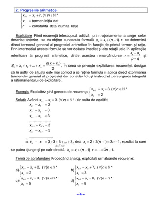
- 5. 2. Progresiile aritmetice ’ā¼ xn ’Ć½1 ’ĆĮ xn ’Ć½ r , (’Ćó)n ’āÄ * ’ā» ’āŁ x1 ’ĆĮ termen ini┼Żial dat ’ā»r ’ĆĮ constant─ā dat─ā numit─ā ra┼Żie ’ā« Explicitare Fiind recuren┼Ż─ā telescopic─ā aditiv─ā, prin ra┼Żionamente analoge celor descrise anterior se va ob┼Żine cunoscuta formul─ā xn ’ĆĮ x1 ’Ć½ (n ’ĆŁ 1) ’āŚ r ce determin─ā direct termenul general al progresiei aritmetice ├«n func┼Żie de primul termen ┼¤i ra┼Żie. Prin intermediul acestei formule se vor deduce imediat ┼¤i alte rela┼Żii utile ├«n aplica┼Żiile a ’ĆŁ aq referitoare la progresii aritmetice, dintre acestea remarc├óndu-se r ’ĆĮ p ┼¤i p’ĆŁq n( x1 ’Ć½ xn ) Sn ’ĆĮ x1 ’Ć½ x2 ’Ć½ ... ’Ć½ xn ’ĆĮ . ├Än ceea ce prive┼¤te explicitarea recuren┼Żei, desigur 2 c─ā ├«n astfel de situa┼Żii este mai comod a se re┼Żine formula ┼¤i aplica direct exprimarea termenului general al progresiei dar consider totu┼¤i instructiv─ā parcurgerea integral─ā a ra┼Żionamentului de explicitare. ’ā¼ x ’ĆĮ xn ’Ć½ 3, (’Ćó)n ’āÄ * Exemplu Explicitez ┼¤irul generat de recuren┼Ża ’āŁ n ’Ć½1 ’ā« x1 ’ĆĮ 2 Solu┼Żie Av├ónd xn’Ć½1 ’ĆŁ xn ’ĆĮ 3, (’Ćó)n ’āÄ * , din suita de egalit─ā┼Żi x2 ’ĆŁ x1 ’ĆĮ 3 x3 ’ĆŁ x 2 ’ĆĮ 3 x 4 ’ĆŁ x3 ’ĆĮ 3 ŌĆ”ŌĆ”ŌĆ”ŌĆ”ŌĆ”ŌĆ” xn ’ĆŁ1 ’ĆŁ xn ’ĆŁ2 ’ĆĮ 3 xn ’ĆŁ xn ’ĆŁ1 ’ĆĮ 3 ____________ (’Ć½) ’ā× xn ’ĆŁ x1 ’ĆĮ 3 ’Ć½ 3 ’Ć½ 3 ’Ć½ ... ’Ć½ 3 , deci xn ’ĆĮ 2 ’Ć½ 3(n ’ĆŁ 1) ’ĆĮ 3n ’ĆŁ 1, rezultat la care de ( n ’ĆŁ1) ori se putea ajunge ┼¤i pe cale direct─ā, xn ’ĆĮ x1 ’Ć½ (n ’ĆŁ 1) ’āŚ r ’ĆĮ ... ’ĆĮ 3n ’ĆŁ 1. Tem─ā de aprofundare Proced├ónd analog, explicita┼Żi urm─ātoarele recuren┼Że: ’ā¼ x ’ĆĮ xn ’Ć½ 2, (’Ćó)n ’āÄ * ’ā¼ x ’ĆĮ xn ’Ć½ 7, (’Ćó)n ’āÄ * a) ’āŁ n ’Ć½1 b) ’āŁ n ’Ć½1 ’ā« x1 ’ĆĮ 2 ’ā« x1 ’ĆĮ 3 ’ā¼ x ’ĆĮ xn ’ĆŁ 3, (’Ćó)n ’āÄ * ’ā¼ x ’ĆĮ xn ’ĆŁ 8, (’Ćó)n ’āÄ * c) ’āŁ n ’Ć½1 d) ’āŁ n ’Ć½1 ’ā« x1 ’ĆĮ 5 ’ā« x1 ’ĆĮ 9 ŌĆō4ŌĆō
- 6. 3. Recuren┼Ża telescopic─ā multiplicativ─ā ’ā¼ xn ’Ć½1 ’ĆĮ xn ’āŚ an , (’Ćó)n ’āÄ * ’ā» ’āŁ x1 ’ĆĮ termen ini┼Żial dat ’ā»(a ) ’ĆŁ ┼¤ir explicit dat ’ā« n n’āÄ * Explicitare Procedura este asem─ān─ātoare cu cea de la recuren┼Ża telescopic─ā aditiv─ā, de aceast─ā dat─ā ├«ns─ā elimin─ārile ce conduc la aflarea expresiei termenului general al ┼¤irului apar la efectuarea produsului iterat corespunz─ātor exprim─ārilor x particulare, respectiv din xn’Ć½1 ’ĆĮ xn ’āŚ an , (’Ćó)n ’āÄ * ’ā× n ’Ć½1 ’ĆĮ an , (’Ćó)n ’āÄ * ┼¤i astfel din xn (’āŚ) n ’ĆŁ1 x2 x x x ’ĆĮ a1, 3 ’ĆĮ a2 , 4 ’ĆĮ a3 , ... , n ’ĆĮ an ’ĆŁ1 ’ā× xn ’ĆĮ x1 ’āŚ ’āĢ ak , produs care ├«n aplica┼Żiile x1 x2 x3 xn ’ĆŁ1 k ’ĆĮ1 propuse se va restr├ónge, uneori prin simplific─āri telescopice, alteori prin exprim─āri combinatorice adecvate. ’ā¼ n2 ’ā» xn ’Ć½1 ’ĆĮ xn ’āŚ , (’Ćó)n ’āÄ * Exemplu Explicitez ┼¤irul generat de recuren┼Ża ’āŁ (n ’Ć½ 1)(n ’Ć½ 2) ’ā»x ’ĆĮ 1 ’ā« 1 xn ’Ć½1 n2 Solu┼Żie Cum ’ĆĮ , (’Ćó)n ’āÄ * , prin particularizare se ob┼Żine xn (n ’Ć½ 1)(n ’Ć½ 2) x2 12 x 22 x4 32 x (n ’ĆŁ 1)2 ’ĆĮ , 3 ’ĆĮ , ’ĆĮ ,..., n ’ĆĮ ┼¤i observ├ónd simplificarea x1 2 ’āŚ 3 x2 3 ’āŚ 4 x3 4 ’āŚ 5 xn ’ĆŁ1 n ’āŚ (n ’Ć½ 1) x x x x 12 22 32 (n ’ĆŁ 1)2 telescopic─ā 2 ’āŚ 3 ’āŚ 4 ’āŚ ... ’āŚ n ’ĆĮ ’āŚ ’āŚ ’āŚ ... ’āŚ , cu ajutorul exprim─ārii x1 x2 x3 xn ’ĆŁ1 2 ’āŚ 3 3 ’āŚ 4 4 ’āŚ 5 n ’āŚ (n ’Ć½ 1) 2 ’āŚ ’üø(n ’ĆŁ 1)!’üØ 2 x 2 factoriale, n ’ĆĮ , rezult─ā ├«n final xn ’ĆĮ 2 . x1 n !’āŚ (n ’Ć½ 1)! n (n ’Ć½ 1) Tem─ā de aprofundare Proced├ónd analog, explicita┼Żi urm─ātoarele recuren┼Że: ’ā¼ n ’ā¼ n(n ’Ć½ 1) ’ā» xn ’Ć½1 ’ĆĮ xn ’āŚ , (’Ćó)n ’āÄ * ’ā» xn ’Ć½1 ’ĆĮ xn ’āŚ , (’Ćó)n ’āÄ * a) ’āŁ n ’Ć½1 b) ’āŁ (n ’Ć½ 2)2 ’ā» x1 ’ĆĮ 1 ’ā« ’ā»x ’ĆĮ 1 ’ā« 1 ’ā¼ n 2 ’Ć½ 3n ’Ć½ 2 ’ā¼ ’ā” 1 ’āČ ’ā» x ’ĆĮ xn ’āŚ 2 , (’Ćó)n ’āÄ * ’ā» xn ’Ć½1 ’ĆĮ xn ’āŚ ’ā¦ 1 ’ĆŁ ’āĘ , (’Ćó)n ’āÄ * c) ’āŁ n ’Ć½1 n ’Ć½ 4n ’Ć½ 3 d) ’āŁ ’ā© 2n ’āĖ ’ā»x ’ĆĮ 1 ’ā»x ’ĆĮ 1 ’ā« 1 ’ā« 1 ŌĆō5ŌĆō
- 7. 4. Progresiile geometrice ’ā¼ xn ’Ć½1 ’ĆĮ xn ’āŚ q, (’Ćó)n ’āÄ * ’ā» ’āŁ x1 ’ĆĮ termen ini┼Żial dat ’ā»q ’ĆĮ constant─ā dat─ā numit─ā ra┼Żie ’ā« Explicitare Acestea fiind generate tot de recuren┼Ża telescopic─ā multiplicativ─ā, prin xn ’Ć½1 x x x x ra┼Żionament analog ’ĆĮ q, (’Ćó)n ’āÄ * ’ā× 2 ’āŚ 3 ’āŚ 4 ’āŚ ... ’āŚ ’āŚ n ’ĆĮ q ’āŚ q ’āŚ q ’āŚ ... ’āŚ q , din xn x1 x2 x3 xn ’ĆŁ1 de ( n ’ĆŁ1) ori care se deduce imediat cunoscuta formul─ā xn ’ĆĮ x1 ’āŚ q n’ĆŁ1 . ’ā¼ x ’ĆĮ 2xn , (’Ćó)n ’āÄ * Exemplu Explicitez ┼¤irul generat de recuren┼Ża ’āŁ n ’Ć½1 ’ā« x1 ’ĆĮ 3 x x x x x ├Än acest caz n ’Ć½1 ’ĆĮ 2, (’Ćó)n ’āÄ * , 2 ’āŚ 3 ’āŚ 4 ’āŚ ... ’āŚ ’āŚ n ’ĆĮ 2 ’āŚ 2 ’āŚ 2 ’āŚ ... ’āŚ 2 ’ā× xn ’ĆĮ 3 ’āŚ 2n ’ĆŁ1 . xn x1 x2 x3 xn ’ĆŁ1 de ( n ’ĆŁ1) ori Tem─ā de aprofundare Proced├ónd analog, explicita┼Żi urm─ātoarele recuren┼Że: ’ā¼ x ’ĆĮ 3 xn , (’Ćó)n ’āÄ * ’ā¼ x ’ĆĮ 10 xn , (’Ćó)n ’āÄ * a) ’āŁ n ’Ć½1 b) ’āŁ n ’Ć½1 ’ā« x1 ’ĆĮ 2 ’ā« x1 ’ĆĮ 7 ’ā¼ 1 ’ā» xn ’Ć½1 ’ĆĮ xn , (’Ćó)n ’āÄ * ’ā¼ x ’ĆĮ ’ĆŁ2xn , (’Ćó)n ’āÄ * c) ’āŁ 2 d) ’āŁ n ’Ć½1 ’ā» x1 ’ĆĮ 3 ’ā« x1 ’ĆĮ 5 ’ā« 5. Recuren┼Ża liniar─ā neomogen─ā de ordin I, cu coeficien┼Żi variabili ’ā¼ xn ’Ć½1 ’ĆĮ an xn ’Ć½ bn , (’Ćó)n ’āÄ * ’ā» ’āŁ x1 ’ĆĮ termen ini┼Żial dat ’ā»(a ) ,(b ) ’ā« n n’āÄ * n n’āÄ * ’ĆŁ ┼¤iruri explicit date Explicitare Explicitarea acestei recuren┼Że se va baza pe transformarea ei ├«ntr-o y recuren┼Ż─ā telescopic─ā aditiv─ā. ├Äntr-adev─ār, introduc├ónd substitu┼Żia an ’ĆĮ n , y1 ’ĆĮ 1, y n ’Ć½1 y rela┼Żia de recuren┼Ż─ā devine xn ’Ć½1 ’ĆĮ n ’āŚ xn ’Ć½ bn , deci xn’Ć½1 ’āŚ y n’Ć½1 ’ĆĮ xn ’āŚ y n ’Ć½ bn ’āŚ y n ’Ć½1 . y n ’Ć½1 Astfel, xn’Ć½1 ’āŚ y n’Ć½1 ’ĆŁ xn ’āŚ y n ’ĆĮ bn ’āŚ y n’Ć½1, (’Ćó)n ’āÄ * ┼¤i particulariz├ónd x2 ’āŚ y 2 ’ĆŁ x1 ’āŚ y1 ’ĆĮ b1 ’āŚ y 2 x3 ’āŚ y 3 ’ĆŁ x2 ’āŚ y 2 ’ĆĮ b2 ’āŚ y 3 ŌĆ”ŌĆ”ŌĆ”ŌĆ”ŌĆ”ŌĆ”ŌĆ”ŌĆ”ŌĆ”ŌĆ” xn ’āŚ y n ’ĆŁ xn ’ĆŁ1 ’āŚ y n ’ĆŁ1 ’ĆĮ bn ’ĆŁ1 ’āŚ y n (’Ć½) n ’ĆŁ1 ’ā× xn ’āŚ y n ’ĆŁ x1 ’āŚ y1 ’ĆĮ ’āź bk ’āŚ y k ’Ć½1 , k ’ĆĮ1 ŌĆō6ŌĆō
- 8. pentru finalizarea explicit─ārii mai fiind necesar─ā doar determinarea ┼¤irului ( y n )n’āÄ * y y y y introdus de substitu┼Żia efectuat─ā. Cum ├«ns─ā 1 ’ĆĮ a1, 2 ’ĆĮ a2 , 3 ’ĆĮ a3 , ... , n ’ĆĮ an , ┼¤i y2 y3 y4 y n ’Ć½1 ’ā” ’āČ ’ā¦ b ’āĘ , xn ’ĆĮ ’ā” ’āĢ ak ’āČ ’āŚ ’ā¦ x1 ’Ć½ ’āź k k ’āĘ , (’Ćó)n ’é│ 2 . Evident n ’ĆŁ1 n ’ĆŁ1 1 y1 ’ĆĮ 1, se ob┼Żine imediat y n ’Ć½1 ’ĆĮ n ’ā¦ ’āĘ ’ā© k ’ĆĮ1 ’āĖ ’ā¦ ’āĢ ak k ’ĆĮ1 ’ā© k ’ĆĮ1 ’āĢ ai ’āĘ i ’ĆĮ1 ’āĖ c─ā ├«n aplica┼Żii este de preferat parcurgerea integral─ā a ra┼Żionamentului expus. ’ā¼ x ’ĆĮ n ’āŚ xn ’Ć½ n !, (’Ćó)n ’āÄ * Exemplu Explicitez ┼¤irul dat de recuren┼Ża ’āŁ n ’Ć½1 ’ā« x1 ’ĆĮ 1 y y Solu┼Żie Not├ónd n ’ĆĮ n , y1 ’ĆĮ 1 ’ā× xn ’Ć½1 ’ĆĮ n ’āŚ xn ’Ć½ n ! ’ā× xn’Ć½1 ’āŚ y n’Ć½1 ’ĆĮ xn ’āŚ y n ’Ć½ n !’āŚ y n ’Ć½1 ┼¤i y n ’Ć½1 y n ’Ć½1 y astfel xn’Ć½1 ’āŚ y n’Ć½1 ’ĆŁ xn ’āŚ y n ’ĆĮ n !’āŚ y n’Ć½1, (’Ćó)n ’āÄ * . Dar din nota┼Żia aplicat─ā, n ’ĆĮ n , cum y n ’Ć½1 y1 y y 1 ’ĆĮ 1 2 ’ĆĮ 2, ..., n ’ĆĮ n ’ā× y n ’Ć½1 ’ĆĮ , deci , xn’Ć½1 ’āŚ y n’Ć½1 ’ĆĮ xn ’āŚ y n ’Ć½ 1, care conduce y2 y3 y n ’Ć½1 n! imediat la xn ’āŚ y n ’ĆĮ x1 ’āŚ y1 ’Ć½ (n ’ĆŁ 1) ┼¤i ├«n final xn ’ĆĮ n ! Tem─ā de aprofundare Proced├ónd analog, explicita┼Żi urm─ātoarele recuren┼Że: ’ā¼ x ’ĆĮ n ’āŚ xn ’Ć½ (n ’Ć½ 1)!, (’Ćó)n ’āÄ * ’ā¼x ’ĆĮ n ’āŚ xn ’Ć½ (n ’Ć½ 2)!, ( ’Ćó)n ’āÄ * a) ’āŁ n ’Ć½1 b) ’āŁ n ’Ć½1 ’ā« x1 ’ĆĮ 1 ’ā« x1 ’ĆĮ1 ’ā¼ 1 1 ’ā¼ xn ’Ć½1 ’ĆĮ n 2 ’āŚ xn ’Ć½ (n !)2, (’Ćó)n ’āÄ * ’ā»x ’ĆĮ ’āŚ xn ’Ć½ , (’Ćó)n ’āÄ * c) ’āŁ d) ’āŁ n ’Ć½1 n n! ’ā« x1 ’ĆĮ 1 ’ā» x1 ’ĆĮ1 ’ā« 6. Recuren┼Ża liniar─ā neomogen─ā de ordin I, cu coeficien┼Żi constan┼Żi ’ā¼ xn ’Ć½1 ’ĆĮ a ’āŚ xn ’Ć½ b, (’Ćó)n ’āÄ * ’ā» ’āŁ x1 ’ĆĮ termen ini┼Żial dat ’ā»a, b ’ĆĮ constante date ’ā« Explicitare Fiind la fel cu recuren┼Ża anterioar─ā, i se poate aplica pentru explicitare acela┼¤i ra┼Żionament, ob┼Żin├ónd la final pentru xn o expresie exponen┼Żial─ā care admite restr├óngere ├«n forma xn ’ĆĮ A ’āŚ an ’Ć½ B . Aceast─ā observa┼Żie permite scurtarea c─āii de explicitare a acestor recuren┼Że, coeficien┼Żii A ┼¤i B put├ónd fi rapid determina┼Żi din sistemul primilor doi termeni ai ┼¤irului. ’ā¼ x ’ĆĮ 2xn ’Ć½ 3, (’Ćó)n ’āÄ * Exemplu Explicitez ┼¤irul dat de recuren┼Ża ’āŁ n ’Ć½1 ’ā« x1 ’ĆĮ 1 ŌĆō7ŌĆō
- 9. Solu┼Żie Av├ónd xn ’ĆĮ A ’āŚ 2n ’Ć½ B , cum x1 ’ĆĮ 1 ┼¤i x2 ’ĆĮ 2x1 ’Ć½ 3 ’ĆĮ 5 , din sistemul ’ā¼2 A ’Ć½ B ’ĆĮ 1 ’āŁ se deduce imediat A ’ĆĮ 2 ┼¤i B ’ĆĮ ’ĆŁ3 , deci xn ’ĆĮ 2n’Ć½1 ’ĆŁ 3 ’ā«4 A ’Ć½ B ’ĆĮ 5 Tem─ā de aprofundare Proced├ónd analog, explicita┼Żi urm─ātoarele recuren┼Że: ’ā¼ x ’ĆĮ 3 xn ’Ć½ 5, (’Ćó)n ’āÄ * ’ā¼ x ’ĆĮ 5 xn ’Ć½ 2, (’Ćó)n ’āÄ * a) ’āŁ n ’Ć½1 b) ’āŁ n ’Ć½1 ’ā« x1 ’ĆĮ 2 ’ā« x1 ’ĆĮ 3 ’ā¼ x ’ĆĮ 2xn ’ĆŁ 3, (’Ćó)n ’āÄ * ’ā¼ x ’ĆĮ ’ĆŁ5 xn ’Ć½ 3, (’Ćó)n ’āÄ * c) ’āŁ n ’Ć½1 d) ’āŁ n ’Ć½1 ’ā« x1 ’ĆĮ 7 ’ā« x1 ’ĆĮ 2 7. Recuren┼Ża liniar─ā omogen─ā de ordin II, cu coeficien┼Żi variabili ’ā¼ xn ’Ć½2 ’ĆĮ an ’āŚ xn ’Ć½1 ’Ć½ bn ’āŚ xn , (’Ćó)n ’āÄ * ’ā» ’āŁ x1 , x2 ’ĆĮ termeni ini┼Żial da┼Żi ’ā»(a ) ,(b ) ’ā« n n’āÄ * n n’āÄ * ’ĆŁ ┼¤iruri explicit date Explicitare Voi prezenta doar un rezultat par┼Żial legat de explicitarea acestui tip de recuren┼Ż─ā. Acesta este con┼Żinut de afirma┼Żia: dac─ā ecua┼Żia t 2 ’ĆŁ an ’āŚ t ’ĆŁ bn ’ĆĮ 0 admite o r─ād─ācin─ā care nu depinde de n ’āÄ * atunci recuren┼Ża devine explicitabil─ā. ├Äntr-adev─ār, dac─ā supranumita ecua┼Żie caracteristic─ā a recuren┼Żei are r─ād─ācinile t1 ’ĆĮ ’üĪ ┼¤i t2 ’ĆĮ ’üón atunci ’üĪ ’Ć½ ’üón ’ĆĮ an ┼¤i ’üĪ ’āŚ ’üón ’ĆĮ ’ĆŁbn . ├Än acest caz vom ob┼Żine xn’Ć½2 ’ĆĮ (’üĪ ’Ć½ ’üón ) ’āŚ xn ’Ć½1 ’ĆŁ ’üĪ’üón ’āŚ xn ’āø xn’Ć½2 ’ĆŁ ’üĪ xn’Ć½1 ’ĆĮ ’üón ’āŚ ( xn ’Ć½1 ’ĆŁ ’üĪ xn ) , recuren┼Ż─ā telescopic─ā multiplicativ─ā care va permite determinarea xn ’Ć½1 ’ĆĮ ’üĪ xn ’Ć½ y n , ob┼Żin├ónd n ’ĆŁ1 y1 ’ĆĮ x2 ’ĆŁ ’üĪ x1 , y n ’ĆĮ ( x2 ’ĆŁ ’üĪ x1 ) ’āŚ ’āĢ ’üók , (’Ćó)n ’é│ 2 . Dar recuren┼Ża xn ’Ć½1 ’ĆĮ ’üĪ xn ’Ć½ y n a fost ┼¤i k ’ĆĮ1 ea tratat─ā anterior ┼¤i particularizat─ā pe aceast─ā situa┼Żie conduce ├«n final la forma ’ā® ’āĢ ’üói ’ā╣ k ’ĆŁ1 ’ā¬x n ’ĆŁ1 ’ā║ explicit─ā xn ’ĆĮ ’üĪ n ’ĆŁ1 ’āŚ ’ā¬ 2 ’Ć½ ( x2 ’ĆŁ ’üĪ x1 )’āź i ’ĆĮ1 k ’ā║ , (’Ćó)n ’é│ 3 . ’ā¬ ’üĪ k ’ĆĮ2 ’üĪ ’ā║ ’ā½ ’ā╗ ’ā¼nx ’ĆĮ 2(2n ’Ć½ 1)xn ’Ć½1 ’ĆŁ 4(n ’Ć½ 1)xn , n ’āÄ * Exemplu: Explicitez ┼¤irul dat de recuren┼Ża ’āŁ n ’Ć½2 ’ā« x1 ’ĆĮ 1 x2 ’ĆĮ 3 , 2(n ’Ć½ 1) Ecua┼Żia caracteristic─ā nt 2 ’ĆŁ 2(2n ’Ć½ 1)t ’Ć½ 4(n ’Ć½ 1) ’ĆĮ 0 are r─ād─ācinile t1 ’ĆĮ 2 , t 2 ’ĆĮ , n deci suntem ├«n condi┼Żii favorabile explicit─ārii. Folosind cunoscutele rela┼Żii dintre r─ād─ācinile ┼¤i coeficien┼Żii ecua┼Żiei de gradul doi, rela┼Żia de recuren┼Ż─ā se va scrie ├«n ’ā® 2(n ’Ć½ 1) ’ā╣ 4(n ’Ć½ 1) x ’ĆŁ 2xn ’Ć½1 2(n ’Ć½ 1) forma xn ’Ć½2 ’ĆĮ ’ā¬2 ’Ć½ ’ā║ ’āŚ xn ’Ć½1 ’ĆŁ ’āŚ xn din care n ’Ć½2 ’ĆĮ . ’ā½ n ’ā╗ n xn ’Ć½1 ’ĆŁ 2xn n ŌĆō8ŌĆō
- 10. De aici se va repeta ra┼Żionamentul ├«nt├ólnit la recuren┼Ża telescopic─ā multiplicativ─ā, ’ā¼ xn ’Ć½1 ’ĆĮ 2xn ’Ć½ n ’āŚ 2n ’ĆŁ1 ob┼Żin├ónd xn’Ć½1 ’ĆŁ 2xn ’ĆĮ n ’āŚ 2 . Dar recuren┼Ża ’āŁ n ’ĆŁ1 este de tip cunoscut, ’ā« x1 ’ĆĮ 1 de aceast─ā dat─ā procedura de explicitare finaliz├ónd cu xn ’ĆĮ (n 2 ’ĆŁ n ’Ć½ 4) ’āŚ 2n’ĆŁ3, (’Ćó)n ’é│ 3 Tem─ā de aprofundare Proced├ónd analog, explicita┼Żi urm─ātoarele recuren┼Że: ’ā¼nx ’ĆĮ 3(2n ’Ć½ 1)xn ’Ć½1 ’ĆŁ 9(n ’Ć½ 1)xn , n ’āÄ * a) ’āŁ n ’Ć½2 ’ā« x1 ’ĆĮ 1 x2 ’ĆĮ 5 , ’ā¼n 2 xn ’Ć½2 ’ĆĮ 2(2n 2 ’Ć½ 2n ’Ć½ 1)xn ’Ć½1 ’ĆŁ 4(n ’Ć½ 1)2 xn , n ’āÄ * b) ’āŁ ’ā« x1 ’ĆĮ 1 x2 ’ĆĮ 3 , ’ā¼n 3 xn ’Ć½2 ’ĆĮ 2(2n 3 ’Ć½ 3n 2 ’Ć½ 3n ’Ć½ 1)xn ’Ć½1 ’ĆŁ 4(n ’Ć½ 1)3 xn , n ’āÄ * c) ’āŁ ’ā« x1 ’ĆĮ 2, x2 ’ĆĮ 5 ’ā¼n 2 xn ’Ć½2 ’ĆĮ 2(2n 2 ’Ć½ 3n ’Ć½ 2)xn ’Ć½1 ’ĆŁ 4(n 2 ’Ć½ 3n ’Ć½ 2)xn , n ’āÄ * d) ’āŁ ’ā« x1 ’ĆĮ 1 x2 ’ĆĮ 5 , 8. Recuren┼Ża liniar─ā omogen─ā de ordin II, cu coeficien┼Żi constan┼Żi ’ā¼ xn ’Ć½2 ’ĆĮ a ’āŚ xn ’Ć½1 ’Ć½ b ’āŚ xn , (’Ćó)n ’āÄ * ’ā» ’āŁ x1 , x2 ’ĆĮ termeni ini┼Żial da┼Żi ’ā»a, b ’ĆĮ constante date ’ā« Explicitare La fel ca ┼¤i cea de ordinul I cu coeficien┼Żi constan┼Żi, ┼¤i aceast─ā recuren┼Ż─ā va permite explicitare imediat─ā, considerente de la recuren┼Ża anterioar─ā pun├ónd ├«n eviden┼Ż─ā urm─ātoarele dou─ā situa┼Żii posibile: I) Ecua┼Żia caracteristic─ā t 2 ’ĆŁ a ’āŚ t ’ĆŁ b ’ĆĮ 0 are r─ād─ācini egale t1 ’ĆĮ t2 ’ĆĮ ’üĪ . ├Än acest caz termenul general este de forma xn ’ĆĮ (nA ’Ć½ B) ’āŚ ’üĪ n II) Ecua┼Żia caracteristic─ā t 2 ’ĆŁ a ’āŚ t ’ĆŁ b ’ĆĮ 0 are r─ād─ācini distincte t1 ’ĆĮ ’üĪ, t2 ’ĆĮ ’üó . ├Än acest caz termenul general este de forma xn ’ĆĮ A ’āŚ ’üĪ n ’Ć½ B ’āŚ ’üó n ├Än ambele situa┼Żii coeficien┼Żii A ┼¤i B se determin─ā din sistemul celor doi termeni ini┼Żial da┼Żi. ’ā¼ x ’ĆĮ 6 xn ’Ć½1 ’ĆŁ 9 xn , n ’āÄ * Exemplu (cazul t1 ’ĆĮ t2 ) Explicitez ┼¤irul dat de recuren┼Ża ’āŁ n ’Ć½2 ’ā« x1 ’ĆĮ 2, x2 ’ĆĮ 7 Ecua┼Żia caracteristic─ā conduce la t1 ’ĆĮ t2 ’ĆĮ 3 , deci xn ’ĆĮ (nA ’Ć½ B) ’āŚ 3n ┼¤i din sistemul ’ā¼( A ’Ć½ B ) ’āŚ 3 ’ĆĮ 2 1 5 termenilor ini┼Żiali, ’āŁ , ob┼Żin A ’ĆĮ , B ’ĆĮ , xn ’ĆĮ (n ’Ć½ 5) ’āŚ 3n’ĆŁ2 ’ā«(2 A ’Ć½ B ) ’āŚ 3 ’ĆĮ 7 2 9 9 ŌĆō9ŌĆō
- 11. ’ā¼ x ’ĆĮ 5 xn ’Ć½1 ’ĆŁ 6 xn , n ’āÄ * Exemplu (cazul t1 ’é╣ t2 ) Explicitez ┼¤irul dat de recuren┼Ża ’āŁ n ’Ć½2 ’ā« x1 ’ĆĮ 4, x2 ’ĆĮ 5 De aceast─ā dat─ā ecua┼Żia caracteristic─ā are r─ād─ācinile t1 ’ĆĮ 2, t2 ’ĆĮ 3 , deci ’ā¼2 A ’Ć½ 3B ’ĆĮ 4 7 xn ’ĆĮ A ’āŚ 2n ’Ć½ B ’āŚ 3n cu ’āŁ , rezult├ónd A ’ĆĮ , B ’ĆĮ ’ĆŁ1, xn ’ĆĮ 7 ’āŚ 2n ’ĆŁ1 ’ĆŁ 3n . ’ā«4 A ’Ć½ 9B ’ĆĮ 5 2 Tem─ā de aprofundare Proced├ónd analog, explicita┼Żi urm─ātoarele recuren┼Że: I) Cazul t1 ’ĆĮ t2 ’ā¼ x ’ĆĮ 4 xn ’Ć½1 ’ĆŁ 4 xn , n ’āÄ * ’ā¼ x ’ĆĮ 10 xn ’Ć½1 ’ĆŁ 25 xn , n ’āÄ * a) ’āŁ n ’Ć½2 b) ’āŁ n ’Ć½2 ’ā« x1 ’ĆĮ 1 x2 ’ĆĮ 2 , ’ā« x1 ’ĆĮ 1 x2 ’ĆĮ 3 , ’ā¼4 x ’ĆĮ 4 xn ’Ć½1 ’ĆŁ xn , n ’āÄ * ’ā¼9 x ’ĆĮ 6 xn ’Ć½1 ’ĆŁ xn , n ’āÄ * c) ’āŁ n ’Ć½2 d) ’āŁ n ’Ć½2 ’ā« x1 ’ĆĮ 1 x2 ’ĆĮ 3 , ’ā« x1 ’ĆĮ 1 x2 ’ĆĮ 2 , II) Cazul t1 ’é╣ t2 ’ā¼ x ’ĆĮ 7 xn ’Ć½1 ’ĆŁ 12xn , n ’āÄ * ’ā¼ x ’ĆĮ 7 xn ’Ć½1 ’ĆŁ 10 xn , n ’āÄ * a) ’āŁ n ’Ć½2 b) ’āŁ n ’Ć½2 ’ā« x1 ’ĆĮ 1 x2 ’ĆĮ 3 , ’ā« x1 ’ĆĮ 2, x2 ’ĆĮ 3 ’ā¼2x ’ĆĮ 5 xn ’Ć½1 ’ĆŁ 2xn , n ’āÄ * ’ā¼2x ’ĆĮ 7 xn ’Ć½1 ’ĆŁ 3 xn , n ’āÄ * c) ’āŁ n ’Ć½2 d) ’āŁ n ’Ć½2 ’ā« x1 ’ĆĮ 1 x2 ’ĆĮ 2 , ’ā« x1 ’ĆĮ 2, x2 ’ĆĮ 5 9. Recuren┼Ża liniar─ā neomogen─ā de ordin II, cu coeficien┼Żi constan┼Żi ’ā¼ xn ’Ć½2 ’ĆĮ a ’āŚ xn ’Ć½1 ’Ć½ b ’āŚ xn ’Ć½ c, (’Ćó)n ’āÄ * ’ā» ’āŁ x1 , x2 ’ĆĮ termeni ini┼Żial da┼Żi ’ā»a, b, c ’ĆĮ constante date ’ā« Explicitare Aceast─ā recuren┼Ż─ā se reduce imediat la tipul anterior, observ├ónd ’ā¼ xn ’Ć½2 ’ĆĮ a ’āŚ xn ’Ć½1 ’Ć½ b ’āŚ xn ’Ć½ c ’āŁ ’ā× ( xn’Ć½3 ’ĆŁ xn’Ć½2 ) ’ĆĮ a ’āŚ ( xn’Ć½2 ’ĆŁ xn’Ć½1 ) ’Ć½ b ’āŚ ( xn’Ć½1 ’ĆŁ xn ) , care este ’ā« xn ’Ć½3 ’ĆĮ a ’āŚ xn ’Ć½2 ’Ć½ b ’āŚ xn ’Ć½1 ’Ć½ c de forma y n’Ć½2 ’ĆĮ a ’āŚ y n ’Ć½1 ’Ć½ b ’āŚ y n cu y n ’ĆĮ xn ’Ć½1 ’ĆŁ xn . Se ob┼Żine astfel xn’Ć½1 ’ĆŁ xn ’ĆĮ y n , recuren┼Ż─ā telescopic─ā aditiv─ā ce va permite finalizarea explicit─ārii. Analiz├ónd forma explicit─ā final─ā vom constata c─ā ┼¤i aceast─ā recuren┼Ż─ā are termenul general de un tip bine determinat, tot ├«n func┼Żie de r─ād─ācinile ecua┼Żiei caracteristice, aceasta fiind ┼¤i de aceast─ā dat─ā tot t 2 ’ĆŁ a ’āŚ t ’ĆŁ b ’ĆĮ 0 . Astfel, vom deosebi situa┼Żiile: I) Ecua┼Żia caracteristic─ā t 2 ’ĆŁ a ’āŚ t ’ĆŁ b ’ĆĮ 0 are r─ād─ācini egale t1 ’ĆĮ t2 ’ĆĮ ’üĪ . ├Än acest caz termenul general este de forma xn ’ĆĮ (nA ’Ć½ B) ’āŚ ’üĪ n ’Ć½ C ŌĆō 10 ŌĆō
- 12. II) Ecua┼Żia caracteristic─ā t 2 ’ĆŁ a ’āŚ t ’ĆŁ b ’ĆĮ 0 are r─ād─ācini distincte t1 ’ĆĮ ’üĪ, t2 ’ĆĮ ’üó . ├Än acest caz termenul general este de forma xn ’ĆĮ A ’āŚ ’üĪ n ’Ć½ B ’āŚ ’üó n ’Ć½ C Coeficien┼Żii A , B ┼¤i C sunt imediat determinabili din sistemul celor doi termeni ini┼Żial da┼Żi ┼¤i al celui de al treilea, ob┼Żinut din recuren┼Ż─ā. ’ā¼ x ’ĆĮ 4 xn ’Ć½1 ’ĆŁ 4 xn ’Ć½ 3, n ’āÄ * Exemplu(cazul t1 ’ĆĮ t2 ) Explicitez ┼¤irul dat de recuren┼Ża ’āŁ n ’Ć½2 ’ā« x1 ’ĆĮ 1 x2 ’ĆĮ 2 , ├Än acest caz ecua┼Żia caracteristic─ā t 2 ’ĆŁ 4t ’Ć½ 4 ’ĆĮ 0 conduce la t1 ’ĆĮ t2 ’ĆĮ 2 , deci xn ’ĆĮ (nA ’Ć½ B) ’āŚ 2n ’Ć½ C ┼¤i din sistemul termenilor ini┼Żiali, inclusiv x3 ’ĆĮ 4x2 ’ĆŁ 4x1 ’Ć½ 3 ’ĆĮ 7 , 3 7 se ob┼Żin A ’ĆĮ , B ’ĆĮ ’ĆŁ , C ’ĆĮ 3 , xn ’ĆĮ (3n ’ĆŁ 7) ’āŚ 2n’ĆŁ2 ’Ć½ 3 . 4 4 ’ā¼ x ’ĆĮ 5 xn ’Ć½1 ’ĆŁ 6 xn ’Ć½ 3, n ’āÄ * Exemplu (cazul t1 ’é╣ t2 ) Explicitez ┼¤irul dat de recuren┼Ża ’āŁ n ’Ć½2 ’ā« x1 ’ĆĮ 1 x2 ’ĆĮ 2 , De aceast─ā dat─ā ecua┼Żia caracteristic─ā are r─ād─ācinile t1 ’ĆĮ 2, t2 ’ĆĮ 3 , deci xn ’ĆĮ A ’āŚ 2n ’Ć½ B ’āŚ 3n ’Ć½ C . Av├ónd x3 ’ĆĮ 5x2 ’ĆŁ 6x1 ’Ć½ 3 ’ĆĮ 7 , din sistemul celor trei termeni 1 3 3n ’ĆŁ 2n ’Ć½1 ’Ć½ 3 cunoscu┼Żi ob┼Żin A ’ĆĮ ’ĆŁ1 B ’ĆĮ , C ’ĆĮ , xn ’ĆĮ , . 2 2 2 Tem─ā de aprofundare Proced├ónd analog, explicita┼Żi urm─ātoarele recuren┼Że: I) Cazul t1 ’ĆĮ t2 ’ā¼ x ’ĆĮ 4 xn ’Ć½1 ’ĆŁ 4 xn ’Ć½ 5, n ’āÄ * ’ā¼ x ’ĆĮ 10 xn ’Ć½1 ’ĆŁ 25 xn ’Ć½ 3, n ’āÄ * a) ’āŁ n ’Ć½2 b) ’āŁ n ’Ć½2 ’ā« x1 ’ĆĮ 1 x2 ’ĆĮ 2 , ’ā« x1 ’ĆĮ 1 x2 ’ĆĮ 3 , ’ā¼4 x ’ĆĮ 4 xn ’Ć½1 ’ĆŁ xn ’Ć½ 7, n ’āÄ * ’ā¼9 x ’ĆĮ 6 xn ’Ć½1 ’ĆŁ xn ’Ć½ 1 n ’āÄ , * c) ’āŁ n ’Ć½2 d) ’āŁ n ’Ć½2 ’ā« x1 ’ĆĮ 1 x2 ’ĆĮ 3 , ’ā« x1 ’ĆĮ 1 x2 ’ĆĮ 2 , II) Cazul t1 ’é╣ t2 ’ā¼ x ’ĆĮ 7 xn ’Ć½1 ’ĆŁ 12xn ’Ć½ 2, n ’āÄ * ’ā¼ x ’ĆĮ 7 xn ’Ć½1 ’ĆŁ 10 xn ’Ć½ 1 n ’āÄ , * a) ’āŁ n ’Ć½2 b) ’āŁ n ’Ć½2 ’ā« x1 ’ĆĮ 1 x2 ’ĆĮ 3 , ’ā« x1 ’ĆĮ 2, x2 ’ĆĮ 3 ’ā¼2x ’ĆĮ 5 xn ’Ć½1 ’ĆŁ 2xn ’Ć½, n ’āÄ * ’ā¼2x ’ĆĮ 7 xn ’Ć½1 ’ĆŁ 3 xn ’Ć½ 4, n ’āÄ * c) ’āŁ n ’Ć½2 d) ’āŁ n ’Ć½2 ’ā« x1 ’ĆĮ 1 x2 ’ĆĮ 2 , ’ā« x1 ’ĆĮ 2, x2 ’ĆĮ 5 10. Recuren┼Że liniare omogene de ordin superior, cu coeficien┼Żi constan┼Żi ’ā¼ xn ’Ć½ p ’ĆĮ a1 ’āŚ xn ’Ć½ p ’ĆŁ1 ’Ć½ a2 ’āŚ xn ’Ć½ p ’ĆŁ2 ’Ć½ ... ’Ć½ ap ’ĆŁ1 ’āŚ xn ’Ć½1 ’Ć½ ap ’āŚ xn , (’Ćó)n ’āÄ *, p ’é│ 3 ’ā» ’āŁ x1 , x2 , ..., x p ’ĆĮ termeni ini┼Żial da┼Żi ’ā» ’ā«a1 , a2 , ..., ap ’ĆĮ constante date ŌĆō 11 ŌĆō
- 13. Explicitare Determinarea explicit─ā a unor astfel de ┼¤iruri se va face la fel ca ┼¤i la suratele lor mai mici prezentate anterior, pa┼¤ii de parcurs fiind urm─ātorii: - se rezolv─ā ecua┼Żia caracteristic─ā t p ’ĆĮ a1 ’āŚ t p’ĆŁ1 ’Ć½ a2 ’āŚ t p’ĆŁ2 ’Ć½ ... ’Ć½ ap’ĆŁ1 ’āŚ t ’Ć½ ap ; - se clasific─ā r─ād─ācinile distincte dup─ā ordinul de multiplicitate; - dac─ā t1 ’āÄ este r─ād─ācin─ā simpl─ā, ea se va prezenta ├«n exprimarea termenului general xn aditiv sub forma A ’āŚ t1n ; - dac─ā t2 ’āÄ este r─ād─ācin─ā dubl─ā, ea se va prezenta ├«n exprimarea termenului general xn aditiv sub forma (nB ’Ć½ C ) ’āŚ t2 ; n - dac─ā t3 ’āÄ este r─ād─ācin─ā tripl─ā, ea se va prezenta ├«n exprimarea termenului general xn aditiv sub forma (n 2D ’Ć½ nE ’Ć½ F ) ’āŚ t3 , etc. n Coeficien┼Żii A, B, C, etc. se ob┼Żin din sistemul termenilor ini┼Żiali ai recuren┼Żei. ’ā¼ x ’ĆĮ 7 xn ’Ć½2 ’ĆŁ 16 xn ’Ć½1 ’Ć½ 12xn , n ’āÄ * Exemplu Explicitez ┼¤irul dat de recuren┼Ża ’āŁ n ’Ć½3 ’ā« x1 ’ĆĮ 1 x2 ’ĆĮ 2, x3 ’ĆĮ 5 , ├Än acest caz ecua┼Żia caracteristic─ā este t 3 ’ĆŁ 7t 2 ’Ć½ 16t ’ĆŁ 12 ’ĆĮ 0 , cu t1 ’ĆĮ 3 r─ād─ācin─ā simpl─ā ┼¤i t2 ’ĆĮ t3 ’ĆĮ 2 r─ād─ācin─ā dubl─ā, deci termenul general al ┼¤irului va avea forma xn ’ĆĮ A ’āŚ 3n ’Ć½ (nB ’Ć½ C ) ’āŚ 2n . Din sistemul termenilor ini┼Żiali se determin─ā coeficien┼Żii, 1 1 1 A ’ĆĮ ,B ’ĆĮ ’ĆŁ ,C ’ĆĮ ┼¤i se ob┼Żine xn ’ĆĮ 3n’ĆŁ1 ’Ć½ (1 ’ĆŁ n) ’āŚ 2n ’ĆŁ2 . 3 4 4 Tem─ā de aprofundare Proced├ónd analog, explicita┼Żi urm─ātoarele recuren┼Że: ’ā¼ x ’ĆĮ 8 xn ’Ć½2 ’ĆŁ 21xn ’Ć½1 ’Ć½ 18 xn , n ’āÄ * ’ā¼ x ’ĆĮ xn ’Ć½2 ’Ć½ 16 xn ’Ć½1 ’Ć½ 20 xn , n ’āÄ * a) ’āŁ n ’Ć½3 b) ’āŁ n ’Ć½3 ’ā« x1 ’ĆĮ 1 x2 ’ĆĮ 5, x3 ’ĆĮ 6 , ’ā« x1 ’ĆĮ 4, x2 ’ĆĮ 5, x3 ’ĆĮ 3 11. Recuren┼Że liniare neomogene de ordin superior, cu coeficien┼Żi constan┼Żi ’ā¼ xn ’Ć½ p ’ĆĮ a1 ’āŚ xn ’Ć½ p ’ĆŁ1 ’Ć½ a2 ’āŚ xn ’Ć½ p ’ĆŁ2 ’Ć½ ... ’Ć½ ap ’ĆŁ1 ’āŚ xn ’Ć½1 ’Ć½ ap ’āŚ xn ’Ć½ b, (’Ćó)n ’āÄ *, p ’é│ 3 ’ā» ’āŁ x1 , x2 , ..., x p ’ĆĮ termeni ini┼Żial da┼Żi ’ā» ’ā«a1 , a2 , ..., ap , b ’ĆĮ constante date Explicitare La fel ca la recuren┼Ża neomogen─ā de ordin doi cu coeficien┼Żi constan┼Żi: - se rezolv─ā ecua┼Żia caracteristic─ā t p ’ĆĮ a1 ’āŚ t p’ĆŁ1 ’Ć½ a2 ’āŚ t p’ĆŁ2 ’Ć½ ... ’Ć½ ap’ĆŁ1 ’āŚ t ’Ć½ ap ; - se clasific─ā r─ād─ācinile distincte dup─ā ordinul de multiplicitate; - dac─ā t1 ’āÄ este r─ād─ācin─ā simpl─ā, ea se va prezenta ├«n exprimarea termenului general xn aditiv sub forma A ’āŚ t1n ; - dac─ā t2 ’āÄ este r─ād─ācin─ā dubl─ā, ea se va prezenta ├«n exprimarea termenului general xn aditiv sub forma (nB ’Ć½ C ) ’āŚ t2 ; n - dac─ā t3 ’āÄ este r─ād─ācin─ā tripl─ā, ea se va prezenta ├«n exprimarea termenului general xn aditiv sub forma (n 2D ’Ć½ nE ’Ć½ F ) ’āŚ t3 , etc. n - se introduce coeficientul termen liber G . Coeficien┼Żii A, B, C,...,G se ob┼Żin din sistemul termenilor ini┼Żiali ai recuren┼Żei. ŌĆō 12 ŌĆō
- 14. ’ā¼ x ’ĆĮ 7 xn ’Ć½2 ’ĆŁ 16 xn ’Ć½1 ’Ć½ 12xn ’ĆŁ 1 n ’āÄ * , Exemplu Explicitez ┼¤irul dat de recuren┼Ża ’āŁ n ’Ć½3 ’ā« x1 ’ĆĮ x2 ’ĆĮ x3 ’ĆĮ 1 Ecua┼Żia caracteristic─ā este t 3 ’ĆŁ 7t 2 ’Ć½ 16t ’ĆŁ 12 ’ĆĮ 0 , cu t1 ’ĆĮ 3 r─ād─ācin─ā simpl─ā ┼¤i t2 ’ĆĮ t3 ’ĆĮ 2 r─ād─ācin─ā dubl─ā, deci termenul general al ┼¤irului va avea forma xn ’ĆĮ A ’āŚ 3n ’Ć½ (nB ’Ć½ C ) ’āŚ 2n ’Ć½ D . Din sistemul termenilor ini┼Żiali ┼¤i x4 ’ĆĮ ... ’ĆĮ 2 se ob┼Żine 1 1 1 1 3n ’ĆŁ1 ’Ć½ (1 ’ĆŁ n ) ’āŚ 2n ’ĆŁ1 ’Ć½ 1 A ’ĆĮ , B ’ĆĮ ’ĆŁ , C ’ĆĮ , D ’ĆĮ , xn ’ĆĮ . 6 4 4 2 2 Tem─ā de aprofundare Proced├ónd analog, explicita┼Żi urm─ātoarele recuren┼Że: ’ā¼ x ’ĆĮ 8 xn ’Ć½2 ’ĆŁ 21xn ’Ć½1 ’Ć½ 18 xn ’ĆŁ 10, n ’āÄ * ’ā¼ x ’ĆĮ xn ’Ć½2 ’Ć½ 16 xn ’Ć½1 ’Ć½ 20 xn ’ĆŁ 15, n ’āÄ * a) ’āŁ n ’Ć½3 b) ’āŁ n ’Ć½3 ’ā« x1 ’ĆĮ 1 x2 ’ĆĮ 1 x3 ’ĆĮ 2 , , ’ā« x1 ’ĆĮ 1 x2 ’ĆĮ 0, x3 ’ĆĮ 0 , 12. Recuren┼Ża omografic─ā cu coeficien┼Żi variabili ’ā¼ a ’āŚ x ’Ć½ bn ’ā» xn ’Ć½1 ’ĆĮ n n , (’Ćó)n ’āÄ * cn ’āŚ xn ’Ć½ d n ’ā» ’ā» ’āŁ x1 ’ĆĮ termen ini┼Żial dat ’ā»(a ) ,(b ) ,(c ) ,(d ) ’ĆŁ ┼¤iruri explicit date ’ā» n n’āÄ * n n’āÄ * n n’āÄ * n n’āÄ * ’ā» ’ā« Explicitare La aceste recuren┼Że vom analiza urm─ātoarele dou─ā cazuri: I) Cazul bn ’ĆĮ 0 Dup─ā cum u┼¤or se va observa, aceast─ā particularitate permite totdeauna an ’āŚ xn 1 d 1 c finalizarea explicit─ārii. ├Äntr-adev─ār xn ’Ć½1 ’ĆĮ ’ā× ’ĆĮ n ’āŚ ’Ć½ n ’ā× not├ónd cn ’āŚ xn ’Ć½ d n xn ’Ć½1 an xn an 1 ’ĆĮ y n recuren┼Ża ia forma y n’Ć½1 ’ĆĮ An ’āŚ y n ’Ć½ Bn care este explicitabil─ā. xn II) Cazul bn ’é╣ 0 Un rezultat par┼Żial ├«n astfel de situa┼Żii este urm─ātorul: - introduc substitu┼Żia cn xn ’Ć½ dn ’ĆĮ y n ’ā× recuren┼Ża ia forma y n’Ć½1 ’āŚ y n ’ĆĮ An ’āŚ y n ’Ć½ Bn z - introduc substitu┼Żia y n ’ĆĮ n ’Ć½1 , z1 ’ĆĮ 1 ’ā× recuren┼Ża ia forma zn’Ć½2 ’ĆĮ An ’āŚ zn’Ć½1 ’Ć½ Bn ’āŚ zn zn cu z1 ’ĆĮ 1 ┼¤i z2 ’ĆĮ ... ’ĆĮ c1 ’āŚ x1 ’Ć½ d1 ’ā× dac─ā ecua┼Żia caracteristic─ā t 2 ’ĆŁ An ’āŚ t ’ĆŁ Bn ’ĆĮ 0 are o r─ād─ācin─ā nedependent─ā de n ’āÄ * atunci zn devine determinabil prin y ’ĆŁ dn zn ’Ć½1 ’ĆŁ dn ’āŚ zn procedur─ā descris─ā anterior ┼¤i astfel xn ’ĆĮ n ’ĆĮ . cn cn ’āŚ zn ŌĆō 13 ŌĆō
- 15. ’ā¼ xn ’ā» xn ’Ć½1 ’ĆĮ Exemplu ( bn ’ĆĮ 0 ) Explicitez ┼¤irul dat de recuren┼Ża ’āŁ n !’āŚ xn ’Ć½ n ’ā»x ’ĆĮ 1 ’ā« 1 1 Cu y n ’ĆĮ recuren┼Ża devine y n’Ć½1 ’ĆĮ ny n ’Ć½ n ! , y1 ’ĆĮ 1 (explicitat─ā anterior) ’ā× y n ’ĆĮ n ! xn 1 ┼¤i astfel xn ’ĆĮ . n! ’ā¼ an xn ’Ć½ bn ’ā» xn ’Ć½1 ’ĆĮ Exemplu ( bn ’é╣ 0 ) Explicitez ┼¤irul dat de recuren┼Ża ’āŁ cn xn ’Ć½ d n cu coeficien┼Żii ’ā»x ’ĆĮ 1 ’ā« 1 an ’ĆĮ n !(’ĆŁn 2 ’Ć½ 3n ’Ć½ 2) , bn ’ĆĮ ’ĆŁn3 ’Ć½ 3n2 ’ĆŁ 2n ’ĆŁ 4 , cn ’ĆĮ (n !)2 ’āŚ n ’āŚ (n ’Ć½ 1) , dn ’ĆĮ n !’āŚ n 2 ’āŚ (n ’Ć½ 1) De┼¤i aceast─ā exprimare apare de-a dreptul descurajant─ā, parcurg├ónd drumul indicat se va ajunge la aceea┼¤i recuren┼Ż─ā zn ’Ć½1 ’ĆĮ nzn ’Ć½ n ! , z1 ’ĆĮ 1 din care se va ob┼Żine zn ’ĆĮ n ! , 1 y n ’ĆĮ n ’Ć½ 1 ┼¤i ├«n final xn ’ĆĮ n! Tem─ā de aprofundare La aceast─ā sec┼Żiune, ca exerci┼Żiu de virtuozitate, propun cititorului s─ā-┼¤i construiasc─ā singur o aplica┼Żie care s─ā permit─ā explicitare ┼¤i bine├«n┼Żeles, s─ā o ┼¤i rezolve ! 13. Recuren┼Ża omografic─ā cu coeficien┼Żi constan┼Żi ’ā¼ a ’āŚ xn ’Ć½ b ’ā» xn ’Ć½1 ’ĆĮ c ’āŚ x ’Ć½ d , (’Ćó)n ’āÄ * ’ā» ’ā» n ’āŁ x1 ’ĆĮ termen ini┼Żial dat ’ā»a, b, c, d ’ĆŁ constante date ’ā» ’ā» ’ā« Explicitare Fiind particularizare a celei anterioare, se vor parcurge ra┼Żionamente analoge, conform cu fiecare din situa┼Żiile: I) Cazul b ’ĆĮ 0 a ’āŚ xn 1 d 1 c 1 Av├ónd xn ’Ć½1 ’ĆĮ ’ā× ’ĆĮ ’āŚ ’Ć½ ’ā× not├ónd ’ĆĮ y n recuren┼Ża ia forma c ’āŚ xn ’Ć½ d xn ’Ć½1 a xn a xn y n ’Ć½1 ’ĆĮ A ’āŚ y n ’Ć½ B care este explicitabil─ā. ├Än aceast─ā situa┼Żie termenul general se va an ob┼Żine de forma xn ’ĆĮ , cu coeficien┼Żii ’üĪ ┼¤i ’üó determinabili din ’üĪ ’āŚ d n ’Ć½ ’üó ’āŚ an sistemul primilor doi termeni, observa┼Żie care poate scurta sensibil explicitarea. ŌĆō 14 ŌĆō
- 16. II) Cazul b ’é╣ 0 ├Än aceast─ā situa┼Żie: - introduc substitu┼Żia cxn ’Ć½ d ’ĆĮ y n ’ā× recuren┼Ża ia forma y n’Ć½1 ’āŚ y n ’ĆĮ A ’āŚ y n ’Ć½ B z - introduc substitu┼Żia y n ’ĆĮ n ’Ć½1 , z1 ’ĆĮ 1 ’ā× recuren┼Ża ia forma zn’Ć½2 ’ĆĮ A ’āŚ zn’Ć½1 ’Ć½ B ’āŚ zn zn z cu z1 ’ĆĮ 1 ┼¤i z2 ’ĆĮ ... ’ĆĮ c ’āŚ x1 ’Ć½ d ’ā× determin zn ’ā× determin y n ’ĆĮ n ’Ć½1 ┼¤i finalizez, zn y ’ĆŁ d zn ’Ć½1 ’ĆŁ d ’āŚ zn ob┼Żin├ónd xn ’ĆĮ n ’ĆĮ . De aceast─ā dat─ā forma termenului general c c ’āŚ zn va fi decis─ā de ordinul de multiplicitate a r─ād─ācinilor ecua┼Żiei t 2 ’ĆŁ A ’āŚ t ’ĆŁ B ’ĆĮ 0 , n ’āŚ’üĪ ’Ć½ ’üó ’üĪ ’āŚ t1n ’Ć½ ’üó ’āŚ t2n respectiv xn ’ĆĮ c├ónd t1 ’ĆĮ t2 ┼¤i xn ’ĆĮ n c├ónd t1 ’é╣ t2 , coeficien┼Żii n ’Ć½’ü¦ t1 ’Ć½ ’ü¦ ’āŚ t2n ’üĪ , ’üó ,’ü¦ fiind determinabili din sistemul primilor trei termeni. ’ā¼ xn ’ā» xn ’Ć½1 ’ĆĮ ,(’Ćó)n ’āÄ * Exemplu ( b ’ĆĮ 0 ) Explicitez ┼¤irul dat de recuren┼Ża ’āŁ 3 xn ’Ć½ 5 ’ā»x ’ĆĮ 1 ’ā« 1 1 1 1 Ob┼Żin ’ĆĮ 5 ’āŚ ’Ć½ 3 ’ā× xn ’ĆĮ , etc. xn ’Ć½1 xn A ’āŚ 3n ’Ć½ B ’ā¼ 5 xn ’ĆŁ 1 ’ā» xn ’Ć½1 ’ĆĮ Exemplu ( b ’é╣ 0, t1 ’ĆĮ t2 ) Explicitez ┼¤irul dat de recuren┼Ża ’āŁ 4 xn ’Ć½ 1 ’ā»x ’ĆĮ 1 ’ā« 1 z Aplicarea substitu┼Żiilor cxn ’Ć½ d ’ĆĮ y n , y n ’ĆĮ n ’Ć½1 , z1 ’ĆĮ 1, va conduce la recuren┼Ż─ā zn omogen─ā de ordin doi. Se ob┼Żin r─ād─ācini ale ecua┼Żiei caracteristice t1 ’ĆĮ t2 ’ĆĮ 3 , etc., n’Ć½2 cu finalizarea xn ’ĆĮ . 2n ’Ć½ 1 ’ā¼ 7 xn ’ĆŁ 4 ’ā» xn ’Ć½1 ’ĆĮ Exemplu ( b ’é╣ 0, t1 ’é╣ t2 ) Explicitez ┼¤irul dat de recuren┼Ża ’āŁ 5 xn ’ĆŁ 2 ’ā»x ’ĆĮ 2 ’ā« 1 z Aplicarea substitu┼Żiilor cxn ’Ć½ d ’ĆĮ y n , y n ’ĆĮ n ’Ć½1 , z1 ’ĆĮ 1, va pune ├«n eviden┼Ż─ā recuren┼Ża zn omogen─ā de ordin doi. Se vor ob┼Żine r─ād─ācini ale ecua┼Żiei caracteristice 3n ’ĆŁ 2n t1 ’ĆĮ 2, t2 ’ĆĮ 3 , etc., cu finalizarea xn ’ĆĮ n . 3 ’ĆŁ 5 ’āŚ 2n ’ĆŁ2 ŌĆō 15 ŌĆō
- 17. Tem─ā de aprofundare Proced├ónd analog, explicita┼Żi urm─ātoarele recuren┼Że: I) Cazul b ’ĆĮ 0 ’ā¼ xn ’ā¼ 2 xn ’ā» xn ’Ć½1 ’ĆĮ ,(’Ćó)n ’āÄ * ’ā» xn ’Ć½1 ’ĆĮ ,(’Ćó)n ’āÄ * a) ’āŁ 5 xn ’Ć½ 2 b) ’āŁ 3 xn ’Ć½ 7 ’ā»x ’ĆĮ 1 ’ā»x ’ĆĮ 2 ’ā« 1 ’ā« 1 II) Cazul b ’é╣ 0, t1 ’ĆĮ t2 ’ā¼ 5 xn ’Ć½ 3 ’ā¼ 3 xn ’ĆŁ 1 ’ā» xn ’Ć½1 ’ĆĮ ,(’Ćó)n ’āÄ * ’ā» xn ’Ć½1 ’ĆĮ ,(’Ćó)n ’āÄ * a) ’āŁ 3 xn ’ĆŁ 1 b) ’āŁ xn ’Ć½ 1 ’ā»x ’ĆĮ 3 ’ā»x ’ĆĮ 2 ’ā« 1 ’ā« 1 III) Cazul b ’é╣ 0, t1 ’é╣ t2 ’ā¼ 4 xn ’ĆŁ 1 ’ā¼ 5 xn ’ĆŁ 2 ’ā» xn ’Ć½1 ’ĆĮ ,(’Ćó)n ’āÄ * ’ā» xn ’Ć½1 ’ĆĮ ,(’Ćó)n ’āÄ * a) ’āŁ 2 xn ’Ć½ 1 b) ’āŁ xn ’Ć½ 2 ’ā»x ’ĆĮ 2 ’ā»x ’ĆĮ 3 ’ā« 1 ’ā« 1 ŌĆō 16 ŌĆō