ºÝºÝߣ

ºÝºÝߣShare a Scribd company logo
Forecasting

DISC 333: SUPPLY CHAIN MANAGEMENT
Forecasting in Operations Function

Forecasting allows predicting future values of a
series based on past observations;

In supply chain the primarily interest is in
forecasting product demand;

Trends, cycles and seasonal variation may be present
in past observations that help us to predict future
demand more closely.
Forecasting Horizon in Supply Chain Planning

 Long (Months / Years)
  Capacity needs, Long-term sales patterns, Growth trends

 Intermediate (Weeks / Months)
  Product family sales, Labor needs, Resource requirements

 Short (Days / Weeks)
  Short-term sales, Shift schedule, Resource requirements
Characteristics of Forecasts

They are usually wrong.
A good forecast is more than a single number.
Aggregate forecasts are more accurate.
The longer the forecast horizon, the less accurate the
forecast will be.
Forecasts should not be used to the exclusion of
known information.
Benefits of Forecasting

Lower inventories
Reduced Stock-outs
Smoother production and supply-chain plans
Reduced production costs
Improved customer service
Etc.
Forecasting Methods

Qualitative (or Subjective) Methods:
 Forecasts based on subjective judgment or opinion
   Sales Force Composites
   Customer Surveys
   Jury of Executive Opinion
   Delphi Method


Quantitative (or Objective) Methods:
 Forecasts are derived based on an analysis of data.
   Time Series Forecasting Models
   Causal or Associative Models
Time Series Forecasting Models

Information can be inferred from the pattern of past
observations and can be used to forecast future values of
the series.

Observations about past values are drawn at discrete points
in time, usually equally spaced.

Time series include various patterns of data:
  Trend
  Seasonality
  Cycles
  Randomness
Simple Moving Average Forecasting Model

A moving average of order N is simply the arithmetic
average of the most recent N observations.
For one step ahead forecasts for most recent N
observations:
                       t −1
       Ft = (1 / N ) ∑ Ai = (1 / N )( At −1 + At − 2 + ... + At − N )
                     i =t − N

       or
                                t
                                                t −1
                                                             
       Ft +1 = (1 / N ) ∑ Ai = (1 / N )  At + ∑ Ai − At − N 
                       i = t − N +1          i =t − N       

       Ft +1 = Ft + (1 / N )[ At − At − N ]
Example: Simple Moving Average

Consider a demand         Period   Demand   MA(3)   MA(6)
process 2, 4, 6, 8,
10, 12, 14, 16, 18, 20,     1        2
22, 24 in which             2        4

there is a definite         3        6
                            4        8        4
trend.                      5        10       6
                            6        12       8

Consider the MA(3)          7        14      10       7
                            8        16      12       9
and MA(6)                   9        18      14      11
                            10       20      16      13
                            11       22      18      15
                            12       24      20      17
Simple Moving Average Forecasting Model (Excel)

Period   Demand Forecast MA(3) Forecast MA(6)           Moving Average MA(3)
  1         2         #N/A          #N/A                30
                                                        25
  2         3         #N/A          #N/A                20


                                                Value
                                                        15
  3        10          5            #N/A                10                                Actual
                                                         5                                Forecast
  4         8          7            #N/A                 0
                                                             1 2 3 4 5 6 7 8 9 10 11 12
  5        12          10           #N/A
                                                                     Data Point
  6        18     12.66666667    8.833333333
  7        24          18           12.5
                                                         Moving Average MA(6)
  8        26     22.66666667    16.33333333
                                                        30
  9        20     23.33333333        18


                                                Value
                                                        20

 10        16     20.66666667    19.33333333            10                                Actual
                                                        0                                 Forecast
 11        22     19.33333333        21
                                                             1 2 3 4 5 6 7 8 9 10 11 12
 12        24     20.66666667        22                              Data Point


                                                Con: Less responsive to changes
                                                in demand.
Weighted Moving Average Forecasting Model

                               t
                 Ft +1 =     ∑w A
                           i =t − N +1
                                         i   i


Allows more emphasis to be placed on recent or past
data.
Weights can be determined by experience of the
forecaster.
Still not responsive enough to track changes in
demand.
Weighted Moving Average (Example)

Perio
  d Demand   Weights   Forecast MA(3)   30

 1    2        0.2                      25

 2    3        0.2                      20
 3    10       0.6
                                        15                                                      Actual
 4    8                      7                                                                  Forecast
                                        10
 5    12                    7.4
 6    18                   10.8          5

 7    24                   14.8         0
                                             1   2   3   4   5   6   7   8   9   10   11   12
 8    26                   20.4
 9    20                    24
10    16                    22
11    22                   18.8
12    24                   20.4
Exponential Smoothing Forecasting Model

Is a sophisticated weighted moving average technique.
Forecast for next period’s demand is the current period’s forecast
adjusted by a fraction of the difference between the current
period’s actual demand and its forecast.
Requires less data to be implemented, thus is more widely
practiced technique.
Suitable for data that show little trend or seasonal patterns.

Ft = α At −1 + (1 − α ) Ft −1
where 0 < α ≤ 1 is the smoothing constant, determines relative weight placed on demand

Ft = Ft −1 − α ( Ft −1 − At −1 )
Ft = Ft −1 − α et −1
Exponential Smoothing Forecasting Model

If we forecast high in period t-1, et-1 is positive and the
adjustment is to decrease the forecast. And vice versa.

If α is large, more weight is given to the current
observation and less weight on past observations,

which results into a forecast that will react quickly to
changes in the demand pattern but may have much
greater variation from period to period.
Exponential Smoothing (Example)

Period   Demand    Forecast
  1        2        #N/A                            Exponential Smoothing
  2        3           2               30
  3        10        2.7               25
  4        8         7.81              20
  5        12       7.943


                               Value
                                       15
  6        18      10.7829                                                                          Actual
                                       10
  7        24      15.83487                                                                         Forecast
                                        5
  8        26     21.550461            0
                                            1   2   3   4   5     6   7      8   9   10   11   12
  9        20     24.6651383
                                                                Data Point
 10        16     21.3995415
 11        22     17.6198624
                                                    α = 0.3 (assumed)
 12        24     20.6859587
Trend Based Exponential Smoothing
           Forecasting Model

          Ft = α At −1 + (1 − α )( Ft −1 + Tt −1 )
         Tt = β ( Ft − Ft −1 ) + (1 − β )Tt −1
          and the trend - adjusted forecast is

         TAFt + m = Ft + mTt

Higher the β higher the emphasis on recent trend
changes.
α & β are determined by trial and error approach.
Linear Trend Forecasting Model

Simple linear regression can be used to fit a line to the time
series historical data.
Linear trend method minimizes the sum of squared deviations
to determine the characteristics of the linear equation:

    ( x1 , y1 ), ( x2 , y2 ),..., ( xn , yn ) be n paired data points for X & Y
    X = Independent Variable
    Y = Dependent Variable
    Suppose a linear relationship exists between X and Y, then
    ∧
    Y = b +b X
         0 1
Linear Trend Forecasting Model

         ∧
where, Y = predicted value of Y
x = time variable
b 0 = intercept of the line, and
b1 = slope of the line


       n∑ ( xy ) − ∑ x ∑ y
b1 =
        n∑ x 2 − (∑ x ) 2


b0   =
       ∑ y −b ∑ x1

             n
Linear Trend Forecasting Model (Example)

What is the trend line and forecast for Period-13 for
the following data?

          Period   Demand   Period   Demand   Period   Demand
            1       1600      5       2500      9       3900
            2       2200      6       3500     10       4700
            3       2000      7       3300     11       4300
            4       1600      8       3200     12       4400
Linear Trend Forecasting Model (Example)

Period Demand                       b1 = [12(282,800) – 78(37,200)] /
  (x)    (y)     x2       xy        [12(650) -78*78]
   1    1600     1       1600
                                       = 286.71
   2    2200     4       4400
   3    2000     9       6000
   4    1600    16       6400     • b0 = [37,000 – 286.71(78)]/12
   5    2500    25      12500          = 1,236.4
   6    3500    36      21000
   7    3300    49      23100
   8    3200    64      25600     Y = 1,236.4 + 286.71 x
   9    3900    81      35100
  10    4700    100     47000
  11    4300    121     47300     F13 = 1236.4 + 286.71 (13) = 4963.5
  12    4400    144     52800
        ∑y =    ∑x2 =    ∑xy =
       37200     650    282,800
Linear Trend Forecasting Model (Example)

Period (x) Demand (y)     Forecast
    1         1600        1523.0769
                                      5000
    2         2200        1809.7902
                                      4500
    3         2000        2096.5035
                                      4000
    4         1600        2383.2168
                                      3500
    5         2500        2669.9301   3000
    6         3500        2956.6434   2500                                                      Actual
    7         3300        3243.3566   2000                                                      Forecast

    8         3200        3530.0699   1500

    9         3900        3816.7832   1000

    10        4700        4103.4965    500

                                        0
    11        4300        4390.2098
                                             1   2   3   4   5   6   7   8   9   10   11   12
    12        4400        4676.9231

Slope       286.7132867
Intercept   1236.363636
Associative Models

One or several external variables are identified that are
related to demand, which are easier to determine than
demand.

Once the relationship between the external variable and
demand is determined, it can be used as a forecasting tool.

Y = Phenomenon to be forecasted

X1 , X2 ,…, Xn = Variables affecting the phenomenon, then

            Y = f(X1 , X2 ,…, X n)
Forecast Accuracy

At = observed demand during periods t, assume {At , t ≥ 1}
Ft = forecast made for period t during period t-1, one step ahead forecast
et = forecast error, then
et = Ft − At
If e1 , e2 ,..., en = forecast errors observed over n periods
                                                   n
MAD = mean absolute deviation = (1 / n)∑ ei
                                                  i =1
                                            n
MSE = mean squared error = (1 / n)∑ ei2
                                           i =1
                                                          n
MAPE = mean absolute percentage error = (1 / n)∑ ei / Di
                                                         i =1
Forecast Accuracy

                                             n
  Running sum of forecast errors (RSFE) =   ∑e
                                            t =1
                                                   t


                     RSFE
  TrackingSignal =
                     MAD


A number of parameters have been defined. Each
one of which provide some sort of advantage over the
other.
Many organizations set targets for Tracking Signal as
a means to improve their forecasts.
Collaborative Planning, Forecasting, and
           Replenishment (CPFR)

The objective of CPFR is to optimize the supply chain
by improving demand forecasting, delivering the
right product at the right time to the right location,
reducing inventories across the supply chains,
avoiding stock-outs, and improving customer
service.
The real value of CPFR comes from an exchange of
forecasting information rather than from more
sophisticated forecasting algorithms to improve
forecasting accuracy.
CPFR Process

More Related Content

Forecasting

  • 1. Forecasting DISC 333: SUPPLY CHAIN MANAGEMENT
  • 2. Forecasting in Operations Function Forecasting allows predicting future values of a series based on past observations; In supply chain the primarily interest is in forecasting product demand; Trends, cycles and seasonal variation may be present in past observations that help us to predict future demand more closely.
  • 3. Forecasting Horizon in Supply Chain Planning Long (Months / Years) Capacity needs, Long-term sales patterns, Growth trends Intermediate (Weeks / Months) Product family sales, Labor needs, Resource requirements Short (Days / Weeks) Short-term sales, Shift schedule, Resource requirements
  • 4. Characteristics of Forecasts They are usually wrong. A good forecast is more than a single number. Aggregate forecasts are more accurate. The longer the forecast horizon, the less accurate the forecast will be. Forecasts should not be used to the exclusion of known information.
  • 5. Benefits of Forecasting Lower inventories Reduced Stock-outs Smoother production and supply-chain plans Reduced production costs Improved customer service Etc.
  • 6. Forecasting Methods Qualitative (or Subjective) Methods: Forecasts based on subjective judgment or opinion Sales Force Composites Customer Surveys Jury of Executive Opinion Delphi Method Quantitative (or Objective) Methods: Forecasts are derived based on an analysis of data. Time Series Forecasting Models Causal or Associative Models
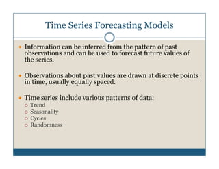
  • 7. Time Series Forecasting Models Information can be inferred from the pattern of past observations and can be used to forecast future values of the series. Observations about past values are drawn at discrete points in time, usually equally spaced. Time series include various patterns of data: Trend Seasonality Cycles Randomness
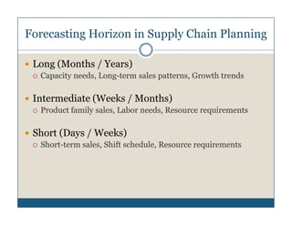
  • 8. Simple Moving Average Forecasting Model A moving average of order N is simply the arithmetic average of the most recent N observations. For one step ahead forecasts for most recent N observations: t −1 Ft = (1 / N ) ∑ Ai = (1 / N )( At −1 + At − 2 + ... + At − N ) i =t − N or t  t −1  Ft +1 = (1 / N ) ∑ Ai = (1 / N )  At + ∑ Ai − At − N  i = t − N +1  i =t − N  Ft +1 = Ft + (1 / N )[ At − At − N ]
  • 9. Example: Simple Moving Average Consider a demand Period Demand MA(3) MA(6) process 2, 4, 6, 8, 10, 12, 14, 16, 18, 20, 1 2 22, 24 in which 2 4 there is a definite 3 6 4 8 4 trend. 5 10 6 6 12 8 Consider the MA(3) 7 14 10 7 8 16 12 9 and MA(6) 9 18 14 11 10 20 16 13 11 22 18 15 12 24 20 17
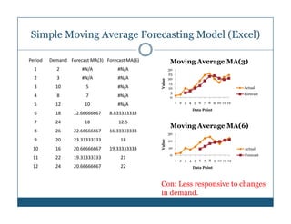
  • 10. Simple Moving Average Forecasting Model (Excel) Period Demand Forecast MA(3) Forecast MA(6) Moving Average MA(3) 1 2 #N/A #N/A 30 25 2 3 #N/A #N/A 20 Value 15 3 10 5 #N/A 10 Actual 5 Forecast 4 8 7 #N/A 0 1 2 3 4 5 6 7 8 9 10 11 12 5 12 10 #N/A Data Point 6 18 12.66666667 8.833333333 7 24 18 12.5 Moving Average MA(6) 8 26 22.66666667 16.33333333 30 9 20 23.33333333 18 Value 20 10 16 20.66666667 19.33333333 10 Actual 0 Forecast 11 22 19.33333333 21 1 2 3 4 5 6 7 8 9 10 11 12 12 24 20.66666667 22 Data Point Con: Less responsive to changes in demand.
  • 11. Weighted Moving Average Forecasting Model t Ft +1 = ∑w A i =t − N +1 i i Allows more emphasis to be placed on recent or past data. Weights can be determined by experience of the forecaster. Still not responsive enough to track changes in demand.
  • 12. Weighted Moving Average (Example) Perio d Demand Weights Forecast MA(3) 30 1 2 0.2 25 2 3 0.2 20 3 10 0.6 15 Actual 4 8 7 Forecast 10 5 12 7.4 6 18 10.8 5 7 24 14.8 0 1 2 3 4 5 6 7 8 9 10 11 12 8 26 20.4 9 20 24 10 16 22 11 22 18.8 12 24 20.4
  • 13. Exponential Smoothing Forecasting Model Is a sophisticated weighted moving average technique. Forecast for next period’s demand is the current period’s forecast adjusted by a fraction of the difference between the current period’s actual demand and its forecast. Requires less data to be implemented, thus is more widely practiced technique. Suitable for data that show little trend or seasonal patterns. Ft = α At −1 + (1 − α ) Ft −1 where 0 < α ≤ 1 is the smoothing constant, determines relative weight placed on demand Ft = Ft −1 − α ( Ft −1 − At −1 ) Ft = Ft −1 − α et −1
  • 14. Exponential Smoothing Forecasting Model If we forecast high in period t-1, et-1 is positive and the adjustment is to decrease the forecast. And vice versa. If α is large, more weight is given to the current observation and less weight on past observations, which results into a forecast that will react quickly to changes in the demand pattern but may have much greater variation from period to period.
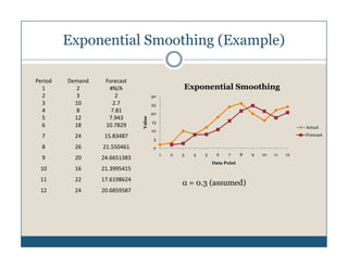
  • 15. Exponential Smoothing (Example) Period Demand Forecast 1 2 #N/A Exponential Smoothing 2 3 2 30 3 10 2.7 25 4 8 7.81 20 5 12 7.943 Value 15 6 18 10.7829 Actual 10 7 24 15.83487 Forecast 5 8 26 21.550461 0 1 2 3 4 5 6 7 8 9 10 11 12 9 20 24.6651383 Data Point 10 16 21.3995415 11 22 17.6198624 α = 0.3 (assumed) 12 24 20.6859587
  • 16. Trend Based Exponential Smoothing Forecasting Model Ft = α At −1 + (1 − α )( Ft −1 + Tt −1 ) Tt = β ( Ft − Ft −1 ) + (1 − β )Tt −1 and the trend - adjusted forecast is TAFt + m = Ft + mTt Higher the β higher the emphasis on recent trend changes. α & β are determined by trial and error approach.
  • 17. Linear Trend Forecasting Model Simple linear regression can be used to fit a line to the time series historical data. Linear trend method minimizes the sum of squared deviations to determine the characteristics of the linear equation: ( x1 , y1 ), ( x2 , y2 ),..., ( xn , yn ) be n paired data points for X & Y X = Independent Variable Y = Dependent Variable Suppose a linear relationship exists between X and Y, then ∧ Y = b +b X 0 1
  • 18. Linear Trend Forecasting Model ∧ where, Y = predicted value of Y x = time variable b 0 = intercept of the line, and b1 = slope of the line n∑ ( xy ) − ∑ x ∑ y b1 = n∑ x 2 − (∑ x ) 2 b0 = ∑ y −b ∑ x1 n
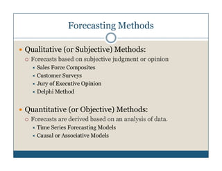
  • 19. Linear Trend Forecasting Model (Example) What is the trend line and forecast for Period-13 for the following data? Period Demand Period Demand Period Demand 1 1600 5 2500 9 3900 2 2200 6 3500 10 4700 3 2000 7 3300 11 4300 4 1600 8 3200 12 4400
  • 20. Linear Trend Forecasting Model (Example) Period Demand b1 = [12(282,800) – 78(37,200)] / (x) (y) x2 xy [12(650) -78*78] 1 1600 1 1600 = 286.71 2 2200 4 4400 3 2000 9 6000 4 1600 16 6400 • b0 = [37,000 – 286.71(78)]/12 5 2500 25 12500 = 1,236.4 6 3500 36 21000 7 3300 49 23100 8 3200 64 25600 Y = 1,236.4 + 286.71 x 9 3900 81 35100 10 4700 100 47000 11 4300 121 47300 F13 = 1236.4 + 286.71 (13) = 4963.5 12 4400 144 52800 ∑y = ∑x2 = ∑xy = 37200 650 282,800
  • 21. Linear Trend Forecasting Model (Example) Period (x) Demand (y) Forecast 1 1600 1523.0769 5000 2 2200 1809.7902 4500 3 2000 2096.5035 4000 4 1600 2383.2168 3500 5 2500 2669.9301 3000 6 3500 2956.6434 2500 Actual 7 3300 3243.3566 2000 Forecast 8 3200 3530.0699 1500 9 3900 3816.7832 1000 10 4700 4103.4965 500 0 11 4300 4390.2098 1 2 3 4 5 6 7 8 9 10 11 12 12 4400 4676.9231 Slope 286.7132867 Intercept 1236.363636
  • 22. Associative Models One or several external variables are identified that are related to demand, which are easier to determine than demand. Once the relationship between the external variable and demand is determined, it can be used as a forecasting tool. Y = Phenomenon to be forecasted X1 , X2 ,…, Xn = Variables affecting the phenomenon, then Y = f(X1 , X2 ,…, X n)
  • 23. Forecast Accuracy At = observed demand during periods t, assume {At , t ≥ 1} Ft = forecast made for period t during period t-1, one step ahead forecast et = forecast error, then et = Ft − At If e1 , e2 ,..., en = forecast errors observed over n periods n MAD = mean absolute deviation = (1 / n)∑ ei i =1 n MSE = mean squared error = (1 / n)∑ ei2 i =1 n MAPE = mean absolute percentage error = (1 / n)∑ ei / Di i =1
  • 24. Forecast Accuracy n Running sum of forecast errors (RSFE) = ∑e t =1 t RSFE TrackingSignal = MAD A number of parameters have been defined. Each one of which provide some sort of advantage over the other. Many organizations set targets for Tracking Signal as a means to improve their forecasts.
  • 25. Collaborative Planning, Forecasting, and Replenishment (CPFR) The objective of CPFR is to optimize the supply chain by improving demand forecasting, delivering the right product at the right time to the right location, reducing inventories across the supply chains, avoiding stock-outs, and improving customer service. The real value of CPFR comes from an exchange of forecasting information rather than from more sophisticated forecasting algorithms to improve forecasting accuracy.