狠狠撸

Introduction?to?Probability?Theory,?
Statistics?and?Distributions
FRM?Level?1?Part?2
Source?Material?‐ https://www.garp.org/#!/frm

Probability?Functions
? Probability?function?p(x),?gives?the?probability?
that?a?discrete?random?variable?will?take?on?a?
value?x?[eg.?p(x)?=?x?/?15?for?X?=?{1,2,3,4,5}??‐>?p(3)?
=?20%.
? Probability?Density?Function?(PDF)?f(x),?gives?the?
probability?of?a?continuous?random?variable.
? Cumulative?distribution?function?(CDF)?F(x),?gives?
the?probability?that?a?random?variable?will?be?less?
than?or?equal?to?a?given?value.

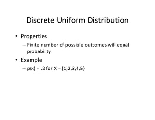
Discrete?Uniform?Distribution
? Properties
– Finite?number?of?possible?outcomes?will?equal?
probability
? Example
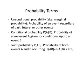
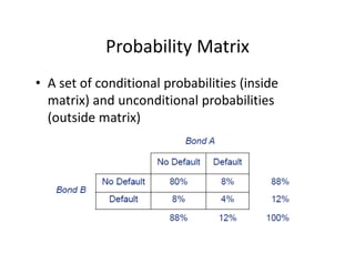
– p(x)?=?.2?for?X?=?{1,2,3,4,5}?

Probability?Terms
? Unconditional?probability?(aka.?marginal?
probability):?Probability?of?an?event?regardless?
of?past,?future,?or?other?events
? Conditional?probability?P(A|B):?Probability?of?
some?event?A?given?(or?conditional?upon)?an?
event?B
? Joint?probability?P(AB):?Probability?of?both?
events?A?and?B?occurring.?P(AB)=P(A|B)?x?P(B)

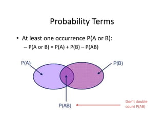
Probability?Terms
? At?least?one?occurrence?P(A?or?B):
– P(A?or?B)?=?P(A)?+?P(B)?– P(AB)
Don’t?double?
count?P(AB)

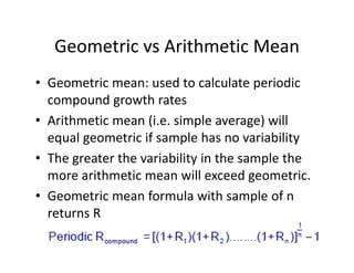
Geometric?vs?Arithmetic?Mean
? Geometric?mean:?used?to?calculate?periodic?
compound?growth?rates
? Arithmetic?mean?(i.e.?simple?average)?will?
equal?geometric?if?sample?has?no?variability?
? The?greater?the?variability?in?the?sample?the?
more?arithmetic?mean?will?exceed?geometric.
? Geometric?mean?formula?with?sample?of?n?
returns?R

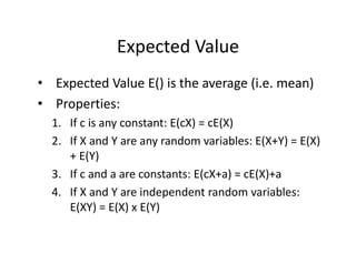
Expected?Value
? Expected?Value?E()?is?the?average?(i.e.?mean)
? Properties:
1. If?c?is?any?constant:?E(cX)?=?cE(X)
2. If?X?and?Y?are?any?random?variables:?E(X+Y)?=?E(X)?
+?E(Y)
3. If?c?and?a?are?constants:?E(cX+a)?=?cE(X)+a?
4. If?X?and?Y?are?independent?random?variables:?
E(XY)?=?E(X)?x?E(Y)?

Variance?and?Standard?Deviation
? Variance?=?σ2 =?E[(X?– E(X))2],?properties:
1. If?c is?constant:?Var(c)?=?0?and?VaR(cX)=c2 x?Var(X)
2. If?c and?a are?constants:?Var(aX+c )?=?a2 x?Var(X)
3. If?c?and?a are?constants:?E(cX+a)?=?cE(X)+a?
4. If?X?and?Y?are?independent?random?variables:?
Var(X+Y)?=?Var(X‐Y)?=?Var(X)?+?Var(Y)
? Standard?Deviation?=?Square?root?of?Variance?
=?σ?=?{E[(X?– E(X))2]}1/2

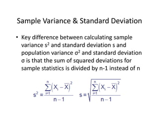
Sample?Variance?&?Standard?Deviation
? Key?difference?between?calculating?sample?
variance?s2 and?standard?deviation?s?and?
population?variance?σ2 and?standard?deviation?
σ?is?that?the?sum?of?squared?deviations?for?
sample?statistics?is?divided?by?n‐1?instead?of?n

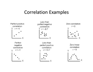
Covariance
? Covariance:?A?measure?of?how?to?variables?move?together.
Cov(X,Y)?=?E[(X‐E(X))(Y‐E(Y))]?=?E(XY)‐E(X)E(Y)?
? Interpretation:
– Values?range?from?negative?to?positive?infinity.?
– Positive?(negative)?covariance?means?when?one?variable?has?
been?above?its?mean?the?other?variable?has?been?above?(below)?
its?mean.
– Units?of?covariance?are?difficult?to?interpret?which?is?why?we?
more?commonly?use?correlation (next?slide)
? Properties:
– If?X?and?Y?are?independent?then?Cov(X,Y)?=?0
– Covariance?of?a?variable?X?with?itself?is?Var(X)
– If?X?and?Y?are?NOT?independent:
? Var(X+Y)?=?Var(X)?+?Var(Y)?+?2(Cov(X,Y)
? Var(X‐Y)?=?Var(X)?+?Var(Y)?‐ 2(Cov(X,Y)

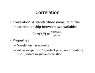
Correlation
? Correlation:?A?standardized?measure?of?the?
linear?relationship?between?two?variables
Corr(X,Y)?
,
? Properties
– Correlation?has?no?units
– Values?range?from?1?(perfect?positive?correlation)?
to?‐1?(perfect?negative?correlation)?

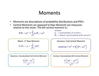
Variance:?2nd?Central?Moment?Mean:?1st Raw?Moment
Moments
? Moments?are?descriptions?of?probability?distributions?and?PDFs:?
? Central?Moments?(as?opposed?to?Raw?Moment)?are?measures?
relative?to?the?mean.?The?kth?central?moment?is::?
Skewness:?Standardized?3rd?Central?Moment Kurtosis:?Standardized?4th?Central?Moment

Skewness
? Positive?(negative)?skew?has?outliers?on?the?
right?(left)?tail
? Skew?absolute?values?>?0.5?are?generally?
considered?significant

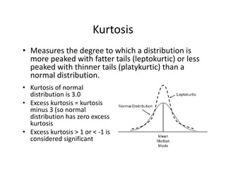
Kurtosis
? Measures?the?degree?to?which?a?distribution?is?
more?peaked?with?fatter?tails?(leptokurtic)?or?less?
peaked?with?thinner?tails?(platykurtic)?than?a?
normal?distribution.
? Kurtosis?of?normal?
distribution?is?3.0
? Excess?kurtosis?=?kurtosis?
minus?3?(so?normal?
distribution?has?zero?excess?
kurtosis
? Excess?kurtosis?>?1?or?<?‐1?is?
considered?significant

Co‐skewness and?Co‐kurtosis
? Similar?to?moments?and?central?moments?for?
means?and?variance,?we?can?identify?cross?
central?moments?for?the?concept?of?
covariance:
– Coskewness:?3rd cross?central?moment
– Cokurtosis:?4th cross?central?moment
? Coskewness and?cokurtosis can?be?captured?
by?incorporating?time‐varying?volatility?and/or?
time‐varying?correlation?into?risk?models

Desirable?Estimator?Properties
? Unbiased:?Expected?value?equal?to?parameter
? Efficient:?Sampling?distribution?has?smallest?
variance?of?all?unbiased?estimators
? Consistent:?Larger?sample?‐>?better?estimator.?
Standard?error?of?estimate?decreases?with?
larger?sample?size
? Linearity:?Used?as?a?linear?function?of?sample?
data

Uniform?Distribution
? Continuous?Uniform?Distribution?(CUD)?is?
defined?over?a?range?that?spans?between?
some?lower?limit,?a,?and?some?upper?limit,?b,?
which?are?the?only?two?parameters.
? Properties
– For?a?random?variable?x?following?a?CUD,?a<x<b
– P(X=x)=0?because?it?is?continuous

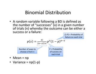
Binomial?Distribution
? A?random?variable?following?a?BD?is?defined?as?
the?number?of?“successes”?(x)?in?a?given?number?
of?trials?(n)?whereby?the?outcome?can?be?either?a?
success?or?a?failure:
!
! !
? Mean?=?np
? Variance?=?np(1‐p)
Number?of?ways?to?
choose?x?from?n
P?=?Probability?
of?success?on?
each?trial
(1‐P)?=?Probability?of?
failure?on?each?trial

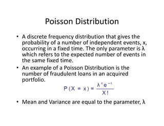
Poisson?Distribution
? A?discrete?frequency?distribution?that?gives?the?
probability?of?a?number?of?independent?events,?x,?
occurring?in?a?fixed?time.?The?only?parameter?is?λ
which?refers?to?the?expected?number?of?events?in?
the?same?fixed?time.?
? An?example?of?a?Poisson?Distribution?is?the?
number?of?fraudulent?loans?in?an?acquired?
portfolio.
? 惭别补苍?补苍诲?痴补谤颈补苍肠别?补谤别?别辩耻补濒?迟辞?迟丑别?辫补谤补尘别迟别谤,?λ

Binomial?vs?Poisson
? If?an?exact?probability?of?an?event?happening?is?
given,?or?implied,?in?the?question,?and?you?are?
asked?to?calculate?the?probability?of?this?event?
happening?k?times?out?of?n,?then?the?Binomial?
Distribution must?be?used.
? If?a?mean?or?average?probability?of?an?event?
happening?per?unit?time/per?page/per?mile?
cycled?etc.,?is?given,?and?you?are?asked?to?
calculate?a?probability?of?n?events?happening?in?a?
given?time/number?of?pages/number?of?miles?
cycled,?then?the?Poisson?Distribution?is?used.?

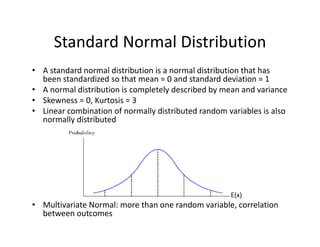
Standard?Normal?Distribution
? A?standard?normal?distribution?is?a?normal?distribution?that?has?
been?standardized?so?that?mean?=?0?and?standard?deviation?=?1
? A?normal?distribution?is?completely?described?by?mean?and?variance
? Skewness =?0,?Kurtosis?=?3
? Linear?combination?of?normally?distributed?random?variables?is?also?
normally?distributed
? Multivariate?Normal:?more?than?one?random?variable,?correlation?
between?outcomes
E(x)

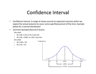
Confidence?Interval
? Confidence?Interval:?A?range?of?values?around?an?expected?outcome?within?we?
expect?the?actual?outcome?to?occur?some?specified?percent?of?the?time.?Example?
below?for?a?normal?distribution
? Common?Standard?Normal?Z‐Scores
Two‐sided?
– N(‐1.96)?=2.5%?so?5%?in?two‐tails?
– N(‐2.58)?=?0.005,?so?1.0%?in?two‐tails?
One‐sided?
– N(‐1.645)?=?5%
– N(‐2.33)?=?1%.?
.?

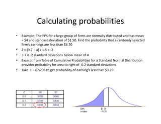
Calculating?probabilities
? Example:?The?EPS?for?a?large?group?of?firms?are?normally?distributed?and?has?mean?
=?$4?and?standard?deviation?of?$1.50.?Find?the?probability?that?a?randomly?selected?
firm’s?earnings?are?less?than?$3.70
? Z?=?(3.7?– 4)?/?1.5?=?‐2
? 3.7?is?.2?standard?deviations?below?mean?of?4
? Excerpt?from?Table?of?Cumulative?Probabilities?for?a?Standard?Normal?Distribution?
provides?probability?for?area?to?right?of?‐0.2?standard?deviations
? Take??1?– 0.5793?to?get?probability?of?earning’s?less?than?$3.70

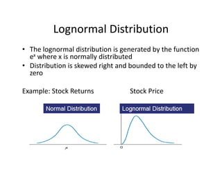
Lognormal?Distribution
? The?lognormal?distribution?is?generated?by?the?function?
ex where?x?is?normally?distributed
? Distribution?is?skewed?right?and?bounded?to?the?left?by?
zero
Example:?Stock?Returns Stock?Price

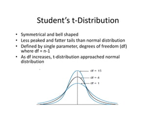
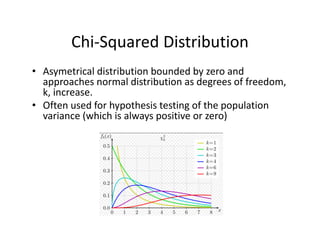
Student’s?t‐Distribution
? Symmetrical?and?bell?shaped
? Less?peaked?and?fatter?tails?than?normal?distribution
? Defined?by?single?parameter,?degrees?of?freedom?(df)?
where?df =?n‐1
? As?df increases,?t‐distribution?approached?normal?
distribution

Chi‐Squared?Distribution
? Asymetrical?distribution?bounded?by?zero?and?
approaches?normal?distribution?as?degrees?of?freedom,?
k,?increase.
? Often?used?for?hypothesis?testing?of?the?population?
variance?(which?is?always?positive?or?zero)

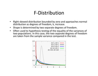
F‐Distribution
? Right?skewed?distribution?bounded?by?zero?and?approaches?normal?
distribution?as?degrees?of?freedom,?k,?increase.
? Shape?is?determined?by?two?separate?degrees?of?freedom.?
? Often?used?to?hypothesis?testing?of?the?equality?of?the?variances?of?
two?populations.?In?this?case,?the?two?separate?degrees?of?freedom?
are?taken?from?the?sample?variance?compared?in?the?test.

Bayes’?Theorem
? Bayes’?Theorem?is?used?to?update?a?given?set?
of?prior?probabilities?for?a?given?event?in?
response?to?the?arrival?of?new?information

Probability?Matrix
? A?set?of?conditional?probabilities?(inside?
matrix)?and?unconditional?probabilities?
(outside?matrix)

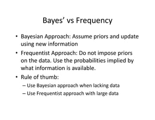
Bayes’?vs?Frequency
? Bayesian?Approach:?Assume?priors?and?update?
using?new?information
? Frequentist?Approach:?Do?not?impose?priors?
on?the?data.?Use?the?probabilities?implied?by?
what?information?is?available.
? Rule?of?thumb:
– Use?Bayesian?approach?when?lacking?data
– Use?Frequentist?approach?with?large?data

Central?Limit?Theorem?and?Sample?
Means

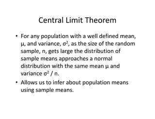
Central?Limit?Theorem
? For?any?population?with?a?well?defined?mean,?
?,?and?variance,?σ2,?as?the?size?of?the?random?
sample,?n,?gets?large?the?distribution?of?
sample?means?approaches?a?normal?
distribution?with?the?same?mean???and?
variance?σ2 /?n.
? Allows?us?to?infer?about?population?means?
using?sample?means.?

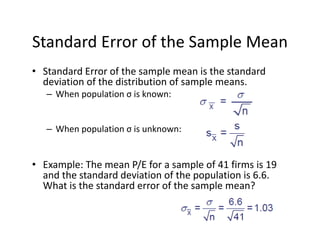
Standard?Error?of?the?Sample?Mean
? Standard?Error?of?the?sample?mean?is?the?standard?
deviation?of?the?distribution?of?sample?means.
– When?population?σ is?known:
– When?population?σ is?unknown:
? Example:?The?mean?P/E?for?a?sample?of?41?firms?is?19?
and?the?standard?deviation?of?the?population?is?6.6.?
What?is?the?standard?error?of?the?sample?mean?

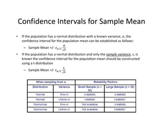
Confidence?Intervals?for?Sample?Mean
? If?the?population?has?a?normal?distribution?with?a?known?variance,?σ,?the?
confidence?interval?for?the?population?mean?can?be?established?as?follows:
– Sample?Mean?+/‐ /
σ
? If?the?population?has?a?normal?distribution?and?only?the?sample?variance,?s,?is?
known?the?confidence?interval?for?the?population?mean?should?be?constructed?
using?a?t‐distribution
– Sample?Mean?+/‐ /
s

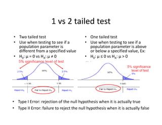
Hypothesis?Testing?and?Confidence?
Intervals

1?vs?2?tailed?test
? Two?tailed?test
? Use?when?testing?to?see?if?a?
population?parameter?is?
different?from?a?specified?value
? H0:?μ =?0?vs?HA:?μ ≠?0
? One?tailed?test
? Use?when?testing?to?see?if?a?
population?parameter?is?above?
or?below?a?specified?value,?Ex:
? H0:?μ ≤?0?vs?HA:?μ >?0
? Type?I?Error:?rejection?of?the?null?hypothesis?when?it?is?actually?true
? Type?II?Error:?failure?to?reject?the?null?hypothesis?when?it?is?actually?false

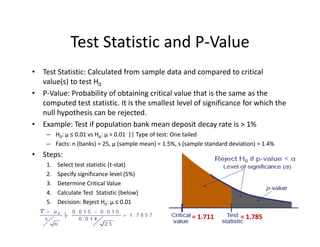
Test?Statistic?and?P‐Value
? Test?Statistic:?Calculated?from?sample?data?and?compared?to?critical?
value(s)?to?test?H0
? P‐Value:?Probability?of?obtaining?critical?value?that?is?the?same?as?the?
computed?test?statistic.?It?is?the?smallest?level?of?significance?for?which?the?
null?hypothesis?can?be?rejected.
? Example:?Test?if?population?bank?mean?deposit?decay?rate?is?>?1%
– H0:?μ ≤?0.01?vs?HA:?μ >?0.01??||?Type?of?test:?One?tailed
– Facts:?n (banks)?=?25,???(sample?mean)?=?1.5%,?s?(sample?standard?deviation)?=?1.4%
? Steps:
1. Select?test?statistic?(t‐stat)
2. Specify?significance?level?(5%)
3. Determine?Critical?Value?
4. Calculate?Test??Statistic?(below)
5. Decision:?Reject?H0:?μ ≤?0.01
=?1.711 =?1.785

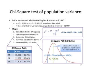
? Is?the?variance?of?a?banks?trading?book?returns?=?0.16%?
– H0:?σ2 =?0.16%?vs?HA:?σ2 ≠?0.16%??||?Type?of?test:?Two?tailed
– Facts:?n?(months)?=?24,?s2 (sample?average?standard?deviation)?=?0.1444%
? Steps:
1. Select?test?statistic?(Chi‐square)
2. Specify?significance?level?(5%)
3. Determine?Critical?Values?
4. Calculate?Test??Statistic?(below)
5. Fail?to?Reject?H0:?μ ≤?0.016
=?(23?x?.14%)?/?.16%?=?20.75
Chi‐Square?test?of?population?variance
df 0.975 0.025
22 10.982 36.781
23 11.689 38.076
24 12.401 39.364
Chi?Square??Table
Chi?Square??PDF?Distribution
11.689?‐ Critical?Values?– 38.076?
X2?=?20.75
Intuition:?X2 is?close?to?n?
(24)?because?hypothesized?
σ2 is?close?to?observed?s2

? An?F‐test?is?any?statistical?test?in?which?the?test?statistic?has?an?F‐distribution?under?the?null?
hypothesis.?
? Often?used?to?determine?the?best?of?two?statistical?models?by?identifying?the?one?that?best?
fits?the?data?they?were?both?estimated?upon.?
? Tests?whether?any?independent?variables?explain?variation?in?dependent?variable.
F‐statistic?with?k?and?n?– (k+1)?degrees?of?freedom
? k?=?number?of?independent?variables??(attributable?to?ESS)
? n?– (k+1)?=?observations?minus?number?of?coefficients
Example:?
? The?ESS?and?SSR?from?a?model?are?500?and?200?respectivly
? Sample?observations?=?100,?Model?has?3?variables
? F?=?(500?/?3)?/?[200?/(100‐3‐1)]?=?80
? Critical?95%?F‐Value?for?3?and?96?df =?2.72?
F‐Test
Numerator?Degrees?
of?Freedom
Denominator?Degrees?
of?Freedom

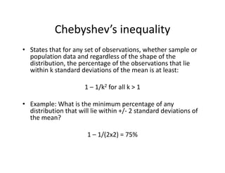
Chebyshev’s inequality
? States?that?for?any?set?of?observations,?whether?sample?or?
population?data?and?regardless?of?the?shape?of?the?
distribution,?the?percentage?of?the?observations?that?lie?
within?k?standard?deviations?of?the?mean?is?at?least:
1?– 1/k2 for?all?k?>?1
? Example:?What?is?the?minimum?percentage?of?any?
distribution?that?will?lie?within?+/‐ 2?standard?deviations?of?
the?mean?
1?– 1/(2x2)?=?75%

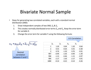
Bivariate?Normal?Sample
? Steps?for?generating?two?correlated?variables,?each?with?a?standard?normal?
distribution?(SND):
1. Draw?independent?samples?of?two?SND,?ZX &?ZY.
2. This?creates?normally?distributed?error?terms?EX and?Ey .Keep?the?error?term?
for?variable?X.
3. Change?the?error?term?for?variable?Y?using?the?following?formula:
Desired?
correlation?
between?X?and?Y
ZX ZY EX EY
1 1.20 0.04 1.20 0.64
2 0.35 ‐0.64 0.35 ‐0.38
3 0.76 ‐1.50 0.76 ‐0.91
997 ‐0.99 ‐1.03 ‐0.99 ‐1.39
998 ‐1.15 ‐0.46 ‐1.15 ‐0.97
999 ‐2.17 2.30 ‐2.17 0.91
1000 ‐0.14 ‐0.22 ‐0.14 ‐0.26
0.5?Correlation

Factor?Models
? Factor?models?can?be?used?to?define?correlations?between?normally?distributed?
variables.?
? Equation?below?is?for?a?one‐factor?model?where?each?Ui has?a?component?
dependent?on?one?common?factor?F?in?addition?to?another?idiosyncratic?factor?Zi
that?is?uncorrelated?with?other?variables.
? Steps?to?construct:
1. Create?the?SND?common?factor?F
2. Choose?a?weight?α for?each?Ui
3. Create?correlations?with?F?(previous?slide)
4. Draw?i?number?of?SND?idiosyncratic?factors?Z
5. Calculate?U?using?equation?to?right
? Advantages?of?Single?Factor?Models:
– Covariance?matrix?is?positive‐semidefinite
– Number?of?correlation?estimations?is?reduced?to?N?from?[Nx(N‐1)]/2
? Capital?Asset?Pricing?Model?(CAPM)?is?well?known?example?of?Single?Factor?Model
Common?
Factor
Idiosyncratic?
Factor

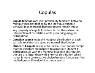
Copulas
? Copula?functions?are?joint?probability?functions?between?
multiple?variables?that?allow?the?individual?variable?
behavior?(e.g.?marginal?distributions)?to?remain?intact
? Key?property?of?copula?functions?is?that?they?allow?the?
introduction?of?correlation?while?preserving?marginal?
distributions
? Gaussian?copula?maps?the?marginal?distribution?of?each?
variable?to?a?bivariate?standard?normal?distribution
? Student’s?t‐copula?is?similar?to?the?Gaussian?copula?except?
that?the?variables?are?mapped?to?a?bivariate?Student?t‐
distribution.?As?with?the?marginal?Student?t‐distribution,?
the?tails?are?fatter?than?with?a?normal?distribution?which?
makes?it?more?conservative?choice?because?it?increases?the?
implied?probability?of?joint?extreme?events

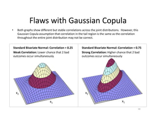
? Both?graphs?show?different?but?stable?correlations?across?the?joint?distributions.??However,?this?
Gaussian?Copula?assumption?that?correlation?in?the?tail?region?is?the?same?as?the?correlation?
throughout?the?entire?joint?distribution?may?not?be?correct.??
50
Standard Bivariate Normal : Correlation = 0.75Standard Bivariate Normal : Correlation = 0.25
x1
x2
x1
x2
Flaws?with?Gaussian?Copula
Standard?Bivariate?Normal:?Correlation?=?0.25
Weak?Correlation:?Lower?chance?that?2?bad?
outcomes?occur?simultaneously.
Standard?Bivariate?Normal:?Correlation?=?0.75
Strong?Correlation:?Higher?chance?that?2?bad?
outcomes?occur?simultaneously

OLS?– Popular?method?of?Linear?Regression
? Linear?relationship?between?dependent?and?independent?variables
? Assumptions
– Independent?variable?uncorrelated?with?error?term
– Expected?value?of?error?term?is?zero
– Variance?of?error?term?is?constant
– Error?term?is?normally?distributed
Error?
Term
Independent?
Variable
Slope?
Coefficient
Intercept
Dependent?
Variable
Sum?of?Squared?
Residuals?(SSR)
Explained??Sum?
of?Squares?(ESS)
Total??…?
(TSS)
Analysis?of?Variance?(ANOVA)

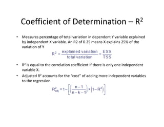
Coefficient?of?Determination?– R2
? Measures?percentage?of?total?variation?in?dependent?Y?variable?explained?
by?independent?X?variable.?An?R2?of?0.25?means?X?explains?25%?of?the?
variation?of?Y
? R2 is?equal?to?the?correlation?coefficient?if?there?is?only?one?independent?
variable?X.
? Adjusted?R2 accounts?for?the?“cost”?of?adding?more?independent?variables?
to?the?regression

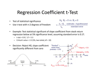
Regression?Coefficient?t‐Test
? Test?of?statistical?significance
? Use?t‐test?with?n‐2?degrees?of?freedom
? Example:?Test?statistical?significant?of?slope?coefficient?from?stock?return?
regression?below?at?5%?significance?level,?assuming?standard?error?is?0.17.
– t‐stat?=?0.9?/?.17?=?5.3
– Critical?t‐value?=?2.2?(5%,?two‐tailed,?df =?10)
? Decision:?Reject?H0,?slope?coefficient?
significantly?different?from?zero?

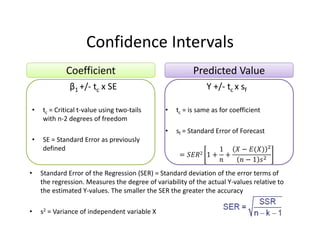
Confidence?Intervals
β1?+/‐ tc x?SE
? tc =?Critical?t‐value?using?two‐tails?
with?n‐2?degrees?of?freedom
? SE?=?Standard?Error?as?previously?
defined
Y?+/‐ tc x?sf
? tc =?is?same?as?for?coefficient
? sf =?Standard?Error?of?Forecast
2 1
1
1
Coefficient Predicted?Value
? Standard?Error?of?the?Regression?(SER)?=?Standard?deviation?of?the?error?terms?of?
the?regression.?Measures?the?degree?of?variability?of?the?actual?Y‐values?relative?to?
the?estimated?Y‐values.?The?smaller?the?SER?the?greater?the?accuracy
? s2 =?Variance?of?independent?variable?X

Gauss‐Markov?Theorem
? If?the?linear?regression?model?assumptions?are?true?and?the?
regression?errors?display?homoskedasticity,?then?the?OLS?
estimator?is?said?to?be?the?Best?Linear?Unbiased?Estimator?
(BLUE).?This?means?that?OLS?has?the?following?four?properties:
1. Estimated?coefficients?have?the?minimum?variance
compared?to?other?methods?of?estimating?the?
coefficients
2. Estimated?coefficients?are?based?on?linear?functions
3. Estimated?coefficients?are?unbiased?
4. Estimate?of?the?variance?of?the?errors?is?unbiased

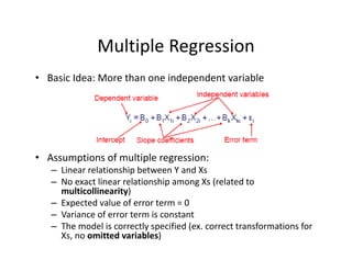
Multiple?Regression
? Basic?Idea:?More?than?one?independent?variable
? Assumptions?of?multiple?regression:
– Linear?relationship?between?Y?and?Xs
– No?exact?linear?relationship?among?Xs (related?to?
multicollinearity)
– Expected?value?of?error?term?=?0
– Variance?of?error?term?is?constant
– The?model?is?correctly?specified?(ex.?correct?transformations?for?
Xs,?no?omitted?variables)

Multicollinearity
? Multicollinearity occurs?when?two?or?more?X?variables?are?highly?
correlated?with?each?other.?
? Effects:
– Inflated?standard?errors,?reduces?t‐stats
– Fail?to?reject?null?hypothesis?too?often?(Type?II?Error)?
– Variables?incorrectly?look?unimportant
? Detection:
– Significant?F‐stat?overall?but?insignificant?t‐stats
– High?correlation?between?X?variables?(if?only?two?Xs).?If?more?than?two?Xs,?low?
correlations?alone?cannot?rule?out?multicolinearilty because?linear?
combinations?may?still?be?highly?correlated.
? Correcting?for?multicollinearity is?typically?accomplished?by?omitting?one?
or?more?independent?variables.?However,?choosing?the?correct?one(s)?to?
omit?can?be?challenging.?Stepwise?regression?is?one?commonly?used?
method.

Omitted?Variable?Bias
? Omitted?Variable?Bias?can?produce?biased?
estimates.?An?omitted?variable?is:
1. Correlated?with?the?movement?of?at?least?one?
independent?variable?and
2. Is?determinant?of?dependent?variable

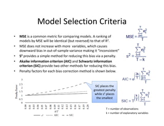
Model?Selection?Criteria
? MSE is?a?common?metric?for?comparing?models.?A?ranking?of?
models?by?MSE?will?be?identical?(but?reversed)?to?that?of?R2.?
? MSE?does?not?increase?with?more??variables,?which?causes?
downward?bias?in?out‐of‐sample?variance?making?it?“inconsistent”?
? S2 provides?a?simple?method?for?reducing?this?bias?via?a?penalty.
? Akaike information?criterion?(AIC)?and?Schwartz?information?
criterion?(SIC)?provide?two?other?methods?for?reducing?this?bias.??
? Penalty?factors?for?each?bias?correction?method?is?shown?below.
SIC?places?the?
greatest?penalty?
while?s2 places?
the?smallest
T?=?number?of?observations
k =?number?of?explanatory?variables

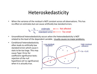
? When?the?variance?of?the?residual?is?NOT?constant?across?all?observations.?This?has?
no?effect?on?estimates?but?can?cause?artificially?low?standard?errors.
? Unconditional?heteroskedasticity occurs?when?the?heteroskedasticity is?NOT?
related?to?the?level?of?the?dependent?variable.??Usually?causes?no?major?problems.
Heteroskedasticity
? Conditional?heteroskedasticity
often?leads?to?artificially?low?
standard?errors?which?cause?t‐
stats?to?be?too?large.?This?may?
cause?Type?I?Error?for?
coefficient?significance?tests:?
rejection?of?the?null?
hypothesis?(of?no?significance)?
when?it?is?actually?true.

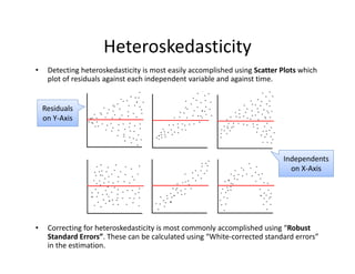
? Detecting?heteroskedasticity is?most?easily?accomplished?using?Scatter?Plots which?
plot?of?residuals?against?each?independent?variable?and?against?time.
? Correcting?for?heteroskedasticity is?most?commonly?accomplished?using?“Robust?
Standard?Errors”.?These?can?be?calculated?using?“White‐corrected?standard?errors”?
in?the?estimation.
Heteroskedasticity
Residuals?
on?Y‐Axis
Independents?
on?X‐Axis

Covariance?Stationarity
? Constant?and?finite?expected?value
? Constant?and?finite?variance
? Constant?and?finite?covariance?between?lags
All?are?examples?of?
non‐stationarity

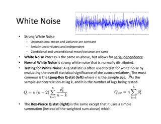
White?Noise
? Strong?White?Noise
– Unconditional?mean?and?variance?are?constant
– Serially?uncorrelated?and?independent
– Conditional?and?unconditional?mean/variance?are?same
? White?Noise?Process?is?the?same?as?above,?but?allows?for?serial?dependence.
? Normal?White?Noise?is?strong?white?noise?that?is?normally?distributed.
? Testing?for?White?Noise:?A?Q‐Statistic?is?often?used?to?test?for?white?noise?by?
evaluating?the?overall?statistical?significance?of?the?autocorrelations.?The?most?
common?is?the?Ljung‐Box?Q‐stat?(left)?where?n?is?the?sample?size,? is?the?
sample?autocorrelation?at?lag?k,?and?h?is?the?number?of?lags?being?tested.
? The?Box‐Pierce?Q‐stat?(right) is?the?same?except?that?it?uses?a?simple?
summation?(instead?of?the?weighted?sum?above)?which?

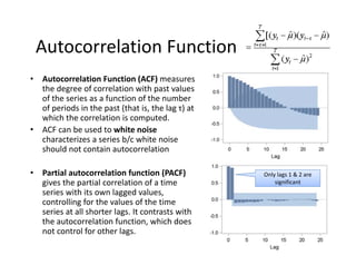
Autocorrelation?Function
? Autocorrelation?Function?(ACF)?measures?
the?degree?of?correlation?with?past?values?
of?the?series?as?a?function?of?the?number?
of?periods?in?the?past?(that?is,?the?lag?τ)?at?
which?the?correlation?is?computed.
? ACF?can?be?used?to?white?noise?
characterizes?a?series?b/c?white?noise?
should?not?contain?autocorrelation
? Partial?autocorrelation?function?(PACF)?
gives?the?partial?correlation?of?a?time?
series?with?its?own?lagged?values,?
controlling?for?the?values?of?the?time?
series?at?all?shorter?lags.?It?contrasts?with?
the?autocorrelation?function,?which?does?
not?control?for?other?lags.
Only?lags?1?&?2?are?
significant

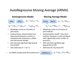
AutoRegressive Moving?Average?(ARMA)
Autoregressive?Model
? Modeling?a?series?as?a?function?of?
past?values
? Gradual?Decay:?Autocorrelation?has?
long?memory?because?current?y?is?
correlated?with?all?previous?y,?albeit?
with?decreasing?strength?
? ACF?will?show?significant?lags?beyond?
that?of?PACF.
? Only?stationary?if?‐1?<?φ <?1
Moving?Average?Model
? Modeling?a?series?as?a?function?of?
past?residuals
? Autocorrelation?Cutoff:?“Very?short?
memory“?because?y?is?only?correlated?
with?a?(generally)?small,?number?of?
previous?y
? PACF?will?show?significant?lags?
beyond?that?of?ACF
? Stationary?for?any?value?of??
AR(1)AR(p) MA(1)MA(q)
ARMA(1,1)? An?ARMA?includes?both?AR?and?MA?terms

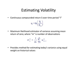
Estimating?Volatility
? Continuous?compounded?return?S?over?time?period?“I”
? Maximum?likelihood?estimator?of?variance?assuming?mean?
return?of?zero;?where?“m”?is?number?of?observations
? Provides?method?for?estimating?today’s?variance?using?equal?
weight?on?historical?values??

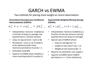
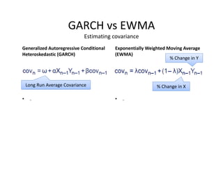
GARCH?vs?EWMA
Two?methods?for?placing?more?weight?on?recent?observations
Generalized?Autoregressive?Conditional?
Heteroskedastic?(GARCH)
? Interpretation:?Variance??modeled?as?
a?function?of?long?run?average,?last?
squared?return,?and?last?variance
? Long?run?avg variance?=?w/(1‐α–β)
? Persistence?=?Sum?α +?β.?If?model?is?
to?be?stationary?(with?mean?
reversion)?persistence?must?be?<?1.
? Estimated?using?MLE
? Superior?to?EWMA?when?volatility?is?
mean?reverting?(which?it?usually?is).?
Exponentially?Weighted?Moving?Average?
(EWMA)
? Interpretation:?Variance?modeled?as?a?
function?of?only?last?variance?and?last?
squared?return?(no?long?run?average)
? Special?case?of?GARCH?where:
– long?run?average (w)?=?0.?
– weight?on?last?return2 (α) =?1‐λ
– Weight?on?last?variance?(β) =?λ
? Requires?no?estimation,?just?supply?λ
? Superior?to?GARCH?when?GARCH?
persistence?is?>=?1?(non‐stationary)

Generalized?Autoregressive?Conditional?
Heteroskedastic?(GARCH)
? .
Exponentially?Weighted?Moving?Average?
(EWMA)
? .
GARCH?vs?EWMA
Estimating?covariance
%?Change?in?Y
%?Change?in?XLong?Run?Average?Covariance

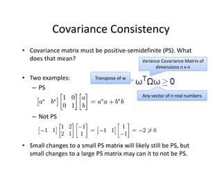
? Covariance?matrix?must?be?positive‐semidefinite (PS).?What?
does?that?mean?
? Two?examples:
– PS
– Not?PS
? Small?changes?to?a?small?PS?matrix?will?likely?still?be?PS,?but?
small?changes?to?a?large?PS?matrix?may?can?it?to?not?be?PS.
Covariance?Consistency
Variance?Covariance?Matrix?of?
dimensions?n?x?n
Any?vector?of?n?real?numbers?
Transpose?of?w

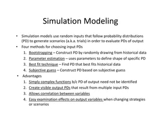
Simulation?Modeling
? Simulation?models?use?random?inputs?that?follow?probability?distributions?
(PD)?to?generate?scenarios?(a.k.a.?trials)?in?order?to?evaluate?PDs?of?output?
? Four?methods?for?choosing?input?PDs
1. Bootstrapping – Construct?PD?by?randomly?drawing?from?historical?data
2. Parameter?estimation – uses?parameters?to?define?shape?of?specific?PD
3. Best?fit?technique – Find?PD?that?best?fits?historical?data?
4. Subjective?guess – Construct?PD?based?on?subjective?guess
? Advantages
1. Simply?complex?functions b/c?PD?of?output?need?not?be?identified
2. Create?visible?output?PDs that?result?from?multiple?input?PDs
3. Allows?correlation?between?variables
4. Easy?examination?effects?on?output?variables?when?changing?strategies?
or?scenarios

Simulation?Modeling
? Incorporating?Correlations?– Common?Approaches
– Correlations?of?inputs?are?implicitly?introduced?by?generating?joint?
scenarios?of?input?variables
– Samples?of?historical?data?are?used?to?define?the?correlations?between?
input?variables?in?the?model
– Correlation?matrix?can?be?specified?as?an?input
? Accuracy
– More?simulations?(i.e.?observations,?trials)?can?increase?accuracy?(see?
formula?for?Standard?Error?of?the?Sample?Mean)
– Estimator?bias?can?be?introduced?via?discretization?error;?the?practice?of?
breaking?the?simulation?into?fixed?time?periods?(ex,?months,?years).?This?
can?be?reduced?by?using?shorter?time?periods,?but?this?also?increases?
cost?of?computation

Inverse?Transform?Method
? Converts?a?random?number?u?that?is?between?0?and?1?to?a?number?from?
the?inverse?of?the?cumulative?distribution?function?(CDF)
? For?discrete?distributions,?the?unit?interval?[0,1]?on?the?y‐axis?(representing?
the?CDF)?is?split?into?segments?based?on?the?cumulative?probabilities?of?
the?discrete?variables
? For?example,?cumulative?probabilities?of?40%?75%?and?100%?could?
correspond?to?values?5,?20,?and?40.

Pseudorandom?Number?Generators
? Reduce?the?variance?of?an?estimate?if?the?
same?sequence?of?random?numbers?is?
reproduced?when?programming?the?model
? Examples:
– Midsquare technique:?square?the?first?random?
number?and?use?middle?digits?for?the?next?random?
number
– Congruential?pseudorandom?number?generator:?
Avoids?the?short?cycle?problem?of?midsquare
technique

狠狠撸

FRM - Level 1 Part 2 - Quantitative Methods including Probability Theory

More Related Content

FRM - Level 1 Part 2 - Quantitative Methods including Probability Theory