�ݺ�ߣ

ENS 491 – Graduation Project (Design)
Proposal
Project Title:
Mathematical Interpretation of the Linguistic Scale
What Does “Significantly More” Mean?
Project #104
Group Members:
Dilara ERŞAHİN - 17671
Sarp UZEL - 18184
Emir ÇAKAR - 16732
Berk ÇETİN - 16508
Supervisor: Kemal KILIÇ
Date: 20.11.2016

2
Table of Contents
INTRODUCTION.....................................................................................................................................................................3
SCALES IN AHP ......................................................................................................................................................................4
1. Linear............................................................................................................................................................................5
2. Power ............................................................................................................................................................................5
3. Root Square..................................................................................................................................................................5
4. Geometric .....................................................................................................................................................................6
5. Inverse Linear..............................................................................................................................................................6
6. Asymptotical................................................................................................................................................................6
7. Balanced.......................................................................................................................................................................6
8. Logarithmic..................................................................................................................................................................6
ELICITING TECHNIQUES IN MCDM ..............................................................................................................................8
1. Analytic Hierarchy Process.......................................................................................................................................8
2. Direct Point Allocation ............................................................................................................................................11
3. Simple Multi Attribute Rating Technique............................................................................................................11
4. SWING Weighting ...................................................................................................................................................12
5. TRADEOFF Weighting...........................................................................................................................................12
CONSISTENCY ISSUE ........................................................................................................................................................12
INDIVIDUALIZATION OF SCALES ...............................................................................................................................14
EXPERIMENTS......................................................................................................................................................................16
1. Distance from Milan.................................................................................................................................................16
2. Games of Chance......................................................................................................................................................16
3. Rainfall in November 2001.....................................................................................................................................17
4. Different Multi Attribute Methods.........................................................................................................................18
5. Visual Psychophysics of Graphical Elements......................................................................................................19
REFERENCES ........................................................................................................................................................................21

3
INTRODUCTION
This report contains the literature review that the project group has done so far during the first
semester of 2016. The project group was given the task to search solutions for inconsistency issue
arose during the implementation of Analytic Hierarchy Process (AHP), since its development. AHP is
a widely used multi-criteria decision making method which is based on generating comparison
matrices by doing pairwise comparisons. It is a known fact in the subject of AHP that as the number of
criteria increases, decision makers are more prone to become more inconsistent. Our claim is that the
inconsistency does not only depend on the decision makers but the scale that is used in the AHP
method. Our hypothesis is that Saaty’s linear scale from 1 to 9 is not a good conversion from verbal
statements to numerical values. The linear scale lacks representing the the meaning of “significantly
more” with the numerical values it contains. The first step for the project group in this project was to
do research on the AHP literature and gather as much information as possible in the planned time
scale.
In Section 2, we present all the information we gathered about the existing scales used in
AHP such as Linear, Power, Root Square, Geometric, Inverse Linear, Logarithmic, Asymptotical,
Balanced. In Section 3, we explained in which ways the different multi-attribute weighting techniques
(SMART,DIRECT,SWING,TRADE-OFF,AHP) differ from each other. In Section 4, we discussed
how consistency ratio measured in AHP, and also how Random Index is calculated for the different
scales. We will also discuss the threshold determined for the matrix to be consistent. In Section 5, we
will examine one of the newest scale tecnique, individual scale. We will display how optimization,
local consistency measurement, transivity can be used for the selection of the scale that should be
implemented. In the last section, Section 6 , we will summarize the experiments that we have studied
so far ; in addition, we will interpret which parts of these existing experiments tecniques can be used
in the experiment we will do in the following semester.

4
SCALES IN AHP
Throughout the years from AHP’s development to the present day, severalscales of judgement
have been used for the implementation of this specific multi-criteria decision making process. The
differencess between the scales emerged from the claim that the linguistic scales may correspond
different numerical values. The verbal statements that correspond to the parameters of the scales are
same for all and are shown in Table 1:
Parameter Order Verbal Statement
1 Equally important
2 Weakly more important
3 Moderately more important
4 Moderately plus more important
5 Strongly more important
6 Strongly plus more important
7 Demonstratedly more important
8 Very, very strongly more important
9 Extremely more important
Table 1: Verbal statements of linguistic scale
Although the scales result in different numerical values for the pairwise comparison matrices,
each one of them is followed by the same procedure,which is the eigenvalue and eigenvetor
computation. The implementation of each scale creates a different average eigenvalue and hence, a
different Random Index for the decision of inconsistency. In our project’s content, we have studied
eight of these judgement scales which are applicable to AHP,which can be listed as Linear, Power,
Root Square, Geometric, Inverse Linear, Asymptotical, Balanced, and Logarithmic.

5
Figure 1 : Judgement scales used in AHP
1. Linear
The Linear scale, developed by Thomas L. Saaty in 1977, is the basis and the original scale
used in the AHP method. The comprehension behind this scale is that the linguistic values have a
linear relationship among them. So, the corresponding numerical values are computed to be from 1
to 9.
2. Power
The Power scale was developed by P. Harker and L. Vargas in 1987, and is based on the
functional relationship of the power law. The linguistic values for this scale refers to the numerical
values of 1, 4, 9, 16, 25, 36, 49, 64, and 81.
3. Root Square
The Root Square scale was formed again by P. Harker and L. Vargas,in 1987. This scale takes
into account the square root relation between our input values. The values of the Linear scale are
taken into their square roots, for the Root Square scale. This refers to the statement of linguistic
scales corresponding to numerical values of 1, √2, √3, 2, √5, √6, √7, √8, and 3.

6
4. Geometric
Freerk A. Lootsma developed the Geometric scale, in 1989. Lootsma claimed that the
geometric relation between the linguistic values and the numerical values would form a more
applicable pairwise comparison matrix for the procedure of AHP. The linguistic values correspond
to the roots of 2, in this scale. So, the numerical values are computed as 1, 2, 4, 8, 16, 32, 64, 128,
and 256.
5. Inverse Linear
The Inverse Linear scale was first introduced by D. Ma and X. Zheng in 1991, and explains
the relationship between the linguistic and numerical values as being inversely linear. This scale,
as the above ones, is based on the parameters x of 1 to 9, and computes the corresponding
numerical values as
9
10−𝑥
, which results in 1, 1.13, 1.29, 1.5, 1.8, 2.25, 3, 4.5, and 9.
6. Asymptotical
The Asymptotical scale, unlike all the other scales of our study, takes numerical values
between 0 and 1. It was developed by F. J. Dodd and H. A. Donegan in 1995. The parameters
from 1 to 9 is inserted in the function tanh−1 (
√3( 𝑥−1)
14
), which results in the numerical values of
0, 0.12, 0.24, 0.36, 0.46, 0.55, 0.63, 0.7, and 0.76.
7. Balanced
The Balanced scale was developed by Ahti A. Salo and Raimo P. Hӓmӓlӓinen, in 1997. Unlike
the other scales, the parameters of x – referred to as weights for this scale- are calculated to be 0.5,
0.55, 0.6, 0.65, 0.7, 0.75, 0.8, 0.85, and 0.9. With a function implementation of
𝑤
1−𝑤
, and the
numerical values are from then on computed as 1, 1.22, 1.5, 1.86, 2.33, 3, 4, 5.67, and 9.
8. Logarithmic
The Logarithmic scale was developed in 2010, by Alessio Ishizaka, Dieter Balkenborg, and
Todd R. Kaplan. By applying the function log2(𝑥 + 1) to the parameters of x from 1 to 9, the
corresponding numerical values were computed to be 1, 1.58, 2, 2.2, 2.58, 2.81, 3, 3.17, and 3.32.

7
The Power and Geometric scales result in higher values of the criterion with the highest
priority. The Asymptotical and Root Square scales result in dominating criterion for the highest
priority, above others.
All of the scales stated above, generates different values for the eigenvalue (λ 𝑚𝑎𝑥) of the
computed matrices and different RI values, the values can be found in Figures 2 and 3.
Figure 2 : Average λ 𝑚𝑎𝑥 values for different scales, and different matrix sizes
Figure 3 : RI values for different scales, and different matrix sizes

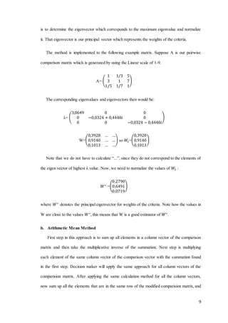
8
The difference in the λ 𝑚𝑎𝑥 and RI values for different matrices were meant to result in a
difference in the inconsistency levels for the scales. The resulting statement was found to be that the
Geometric and Inverse Linear, and Logarithmic scales are less sensitive to inconsistency compared to
the other scales. On the other hand, the Root Square scale was found to be the most sensitive, or the
least tolerant, to inconsistency. The consistency issue will be explained further in the section 4,
Consistency Issue.
ELICITING TECHNIQUES IN MCDM
There have been developed severalMCDM methods, since the decision making became
crucial for both our daily lives and for making critical decisions for companies. Throughout our
project, we have studied other applicable MCDM methods, along with AHP. The scope of our study
for the methods included AHP, DIRECT,SMART, SWING, and TRADEOFF. Each of these methods
have different approaches to interpreting weights of the criteria.
1. Analytic Hierarchy Process
The AHP method, developed by Thomas L. Saaty in 1977, provides ease in the selection of an
alternative where all the alternatives have multiple criteria. The decision maker(DM) is first asked
to rank the attributes in a hierarchical manner. The next step is to compare the importance of the
attributes over one another. The comparison is performed by a pairwise comparison matrix, in
which the DM inserts values from a 1-9 Linear scale, corresponding to the verbal statements of
preference. The weight values are computed in three different ways; the original way is using the
eigenvector method, the heuristic methods are the arithmetic and geometric mean methods.
a. Eigenvector Method
Whereas calculating the weights of each criterion with using the eigenvector method takes
more time than the heuristic methods, it converges to more accurate weighting results. In this
approach there are basically 3 steps which the decision maker should consider. First step is to
find the eigenvalues of the corresponding square comparison matrix. Secondly , the
eigenvectors are calculated by using the eigenvalues calculated in the first step . The last step

9
is to determine the eigenvector which corresponds to the maximum eigenvalue and normalize
it. That eigenvector is our principal vector which represents the weights of the criteria.
The method is implemented to the following example matrix. Suppose A is our pairwise
comparison matrix which is generated by using the Linear scale of 1-9.
A= (
1 1/3 5
3 1 7
1/5 1/7 1
)
The corresponding eigenvalues and eigenvectors then would be:
λ= (
3,0649 0 0
0 −0,0324 + 0,4448𝑖 0
0 0 −0,0324 − 0,4448𝑖
)
W=(
0,3928 … …
0,9140 … …
0,1013 … …
) so 𝑊1=(
0,3928
0,9140
0,1013
)
Note that we do not have to calculate “...”, since they do not correspond to the elements of
the eigen vector of highest λ value. Now, we need to normalize the values of 𝑊1 :
𝑊∗ =(
0,2790
0,6491
0,0719
)
where 𝑊∗ denotes the principal eigenvector for weights of the criteria. Note how the values in
W are close to the values 𝑊∗, this means that W is a good estimator of 𝑊∗.
b. Arithmetic Mean Method
First step in this approach is to sum up all elements in a column vector of the comparison
matrix and then take the multiplicative inverse of the summation. Next step is multiplying
each element of the same column vector of the comparison vector with the summation found
in the first step. Decision maker will apply the same approach for all column vectors of the
comparision matrix. After applying the same calculation method for all the column vectors,
now sum up all the elements that are in the same row of the modified comparision matrix, and

10
multiply the summation found in the row operation with
1
𝑛
where n≥1 , denotes the size of
the square matrix to create priority vector. The elements of the priority vector now represents
the weights of the each corresponding criterion. This method is also called normalized
principal eigenvector, since we are not directly calculating the eigenvector of the comparison
matrix, but relaxing the problem and applying heuristic methods to estimate the eigen vector.
Let us perform this method on the same matrix in the section Eigenvector Method.
A= (
1 1/3 5
3 1 7
1/5 1/7 1
)
Sum=
21
5
31
21
13
After applying the first step, our matrix becomes:
A= (
5/21 7/31 5/13
15/21 21/31 7/13
1/21 3/31 1/13
)
Sum= 1 1 1
The corresponding primary vector would then be:
W=
1
3
*(
5
21
+
7
31
+
5
13
15
21
+
21
31
+
7
13
1
21
+
3
31
+
1
31
)=(
0,2828
0,6434
0,0738
)
c. Geometric Mean Method
This method mainly depends on taking the geometrical average of the row vectors of the
comparison matrix, this is why it is called the heuristic geometric weight calculation. Again
the purpose of using such a method is to estimate the eigenvector to determine the weights of
each criterion. First step is to multiply all the elements in a row vector of the comparison
matrix, and take the 𝑛 𝑡ℎ root of the multiplication. Repeat the same step for all row vectors of
the comparison matrix. After finishing the calculations for each row vector, sum up all the

11
elements of the nx1 vector that is structured by taking the 𝑛 𝑡ℎ root of each row product and
normalize the nx1 vector to find a good estimator for the eigenvector.
Suppose our comparison matrix A and the step results are as followed:
A=(
1 1/8 1/3
8 1 3
3 1/3 1
)
P = (
0,347
2,884
1
)
W = (
0,082
0,682
0,236
)
Sum= 1
where W denotes the pricipal eigenvector.
From this procedure the attribute weights are computed. The final procedure of AHP is to
measure the consistency or inconsistency level of the resulting matrices. The AHP method,
accepts an exceeding of 10% from the specified Random Index value.
2. Direct Point Allocation
In DIRECT method, the decision maker(DM) is supposed to allocate 100 points among all the
criteria –also defined by the decision maker. In other words, the DM has to give scores to each
criteria and the summation of these scores will add up to 100 points. The criteria should be ranked
from the best to the worst, so that the highest score must be assigned to the most important
criterion, and the following least important criteria will have lower scores. The assigned points are
considered to be the attribute weights.
3. Simple Multi Attribute Rating Technique
The SMART method, pioneered by Ward Edwards in 1971, consists of two steps in the
interpretation of the weights for the criteria. First step for the DM is to rank the importance of the
possible changes in the criteria from the worst attribute levels to the best levels. The following

12
step is to make ratio estimation of the importance of each criteria relative to the one ranked as the
lowest importance. The second step usually begins by assigning 10 points to the criterion with the
lowest importance and continues by assigning 10 points upwards to the relative importance of the
remaining criteria. At the end, normalization is done on the points in order to get the weights of
attributes.
4. SWING Weighting
In the SWING method, which was developed by Von Winterfelt and Ward Edwards in 1986,
the decision maker considers a hypothetical attribute in which all criteria are at their worst levels
and assigns 100 points to the criteria that he/she wants to change it to its best level in the first
hand. Next, the DM needs to decide which criterion should be changed to its best level as the
second, and assigns a point to this criterion which is less than 100, and the same step is repeated
until each criterion has its own point assigned. Finally, the points are normalized so that their
summation would be equal to 1, and these resulting normalized values are considered to be the
weights of the attribute.
5. TRADEOFF Weighting
In TRADEOFF method, the decision maker is given a consideration of a situation in which
he/she needs to decide between two alternatives, having only two attributes that are different in
values. The DM is supposed to rank the two attributes in his/her preferred importance order, and
then change the value of one attribute in a way to equalize the preference of the alternatives.
Finally, the attribute weights are computed in the same manner as AHP.
CONSISTENCY ISSUE
Thomas L. Saaty proposed the AHP method with the implementation of the eigenvector
method for the evaluation of pairwise comparison matrices. Although there are other heuristic method
for pairwise matrix evaluation, we preferred to use the method Saaty instructed.
Stated by the Perron-Frobenius Theorem, for a given non-negative square matrix A there
exists its eigenvalues (𝜆 𝑚𝑎𝑥) in which one of them is positive and either greather than or equal to the
other eigenvalues. And for that specific maximum eigenvalue, there is always a corresponding positive

13
eigenvector (w). The eigenvector w is referred to as the matrix Frobenius root for the equation below
(Alonso & Lamata, 2006):
Aw = 𝜆 𝑚𝑎𝑥 w
After computation of the eigenvalue, a check for consistency is needed in order to
accept/reject the pairwise comparison matrix. In order to compute the unit of measurement for
consistency, we first need to obtain two different indexes: consistency index and the random index.
The consistency index is measured as;
CI =
𝜆 𝑚𝑎𝑥−𝑛
𝑛−1
where 𝜆 𝑚𝑎𝑥 is the maximum eigenvalue of the specific matrix, and n refers to the dimension of the
n×n matrix. The random index is unique to the scale used and the value of n of the pairwise
comparison matrices. It is already stated for each judgement scale and it is basically the average of the
CI values of randomly generated matrices of that scale. The RI values for different scales we have
studied is shown in the Figure 3. After obtaining the values for CI and RI, the consistency ratio is
calculated by the function:
𝐶𝑅 =
𝐶𝐼
𝑅𝐼
For the AHP eigenvector method, the acceptance of the matrices depend on the value that CR
takes. If the CI value exceeds the RI by more than 10%, Saaty states that the matrix can not be
accepted as consistent (Alonso & Lamata, 2006).
In order for a matrix to be out of the tolerance zone for consistency, two specifications should
be fulfilled; the matrix in its structure should possess the transitivity property, and the 𝜆 𝑚𝑎𝑥 value
should be in the specified interval of acceptance. For a matrix A of n×n having matrix entries of 𝑎 𝑖𝑗,
transitivity states that the equation 𝑎 𝑖 𝑗 ∗ 𝑎𝑗𝑘 = 𝑎 𝑖𝑘 should be satisfied (Bozóki & Rapcsák,2007).
This property is violated mostly by the decision makers’ selection of numerical values from the given
scale. Although there exists a great amount of literature in which it is stated that the inconsistency
occurs only due to the decision makers behaviours. What we claim as a project team is that the
inconsistency can not only be due to the decision makers, but the selection of the scale as well. Hence,
our objective is to minimize the inconsistency as much as possible, either by selecting the most

14
suitable scale from the literature or developing a new scale which will enable us to decrease the
inconsistency level.
INDIVIDUALIZATION OF SCALES
Although being widely used, the AHP method of Saaty’s is exposed to several critics in terms
of the consistency issue it forms. Alonso and Lamata (2006) criticized the 10% limit of acceptance for
CR value of the AHP method for being too strict. They have suggested that the decision makers
themselves should decide on the level of consistency for their specific problem in hand. Dong et al.
(2013) criticized is the procedure of letting the decision maker assign pairwise comparison matrix
entries from a numerical scale of 1 to 9. What they have claimed is, the decision makers should form
up a linguistic pairwise comparison matrix.
In their study, Dong et al.(2013) proposed an individualized scale, which is formed by taking
the verbal statements for preference from the decision makers and converting those statements into
numerical values by a function. The linguistic scale they have defined for AHP is:
Figure 4: Linguistic scale
They have proposed two functions: 𝑓𝑖 which converts the linguistic entry to a numerival value,
and 𝑓−1
𝑖 which converts numerical values to linguistic entries. They have stated limits for the 𝑓𝑖
function:
LB < 𝑓𝑖 < UB and 𝑓𝑖 < 𝑓𝑖+1

15
where LB is the lower bound and UB is the upper bound, the bounds are calculated by the minimum
and maximum values of 𝑆𝑖 -for LB and UB respectively- of the Linear, Geometric, Inverse Linear, and
Balanced scales used in AHP.
𝑆0 𝑆1 ... 𝑆16
Linear 1/9 1/8 ... 9
Geometric 1/256 1/128 ... 256
Inverse Linear 1/9 1/ 4.5 ... 9
Balanced 1/9 1/5.67 ... 9
Table 2: Linguistic scale values for different judgement scales
The decision maker is asked to form a linguistic pairwise comparison matrix by assigning
values to only the upper part of the diagonal entries. For a 3x3 matrix, the decision makers matrix
would look like:
[
1 𝑠 𝑟 𝑒 𝑟𝑡
1
𝑠 𝑟
⁄ 1 𝑠 𝑡
1
𝑒 𝑟𝑡
⁄ 1
𝑠 𝑡
⁄ 1
]
By their individualized scale method, Dong et al. aimed to reduce the inconsistency level
mainly by obtaining the transitivity property for their matrices. Therefore, their method needs an
estimation of the 𝒆 𝒓𝒕 values as (Dong et al., 2013):
𝑒 𝑟𝑡̂ = 𝑓−1(𝑓( 𝑠 𝑟) ∗ 𝑓( 𝑠 𝑡))
Then, the objective function becomes minimizing the deviation between 𝑒 𝑟𝑡 and 𝑒 𝑟𝑡̂ values,
which is stated as:
𝑑( ∑ 𝑒 𝑟𝑡
16
𝑟,𝑡=0
, 𝑒 𝑟𝑡̂ )
To sum up, individualized scales are aiming to minimize the inconsistency level and enables
the selection of the most suitable scale for a specific decision maker.

16
EXPERIMENTS
This project aims to select or develop a scale applicable to AHP, which will minimize the
inconsistency resulted by the Linear scale of Saaty. In order to achieve this goal, the first step of our
project was stated to be research on literature. The literature on this issue includes both theoretical and
psychophysical experiments.
1. Distance from Milan
Performed by Bernoscani, Choirat, and Seri (2010), this experiment is based on estimation of
distances from a reference point. A total number of 69 subjects performed the experiment. The
natural scale to compare the result of subjects were based on actual kilometer values between
Milan and the cities Naples, Venice, Rome, Turin, and Palermo. The subjects were asked to
compare the cities in pairs and state their estimation on the ratios of distances. The natural scale is
shown in Figure 5.
Figure 5: Natural scale of the experiment Distance from Milan
2. Games of Chance
The Games of Chance experiment was also done by Bernoscani, Choirat, and Seri. This time,
the 69 subjects were asked to estimate the probability ratios of a game result, which is totally
depended on chance of the players. The games of chance that are included in this experiment are
taking cards out of a deck of 52, and rolling a 6-sided dice. Figure 6 shows the specific
probabilities being asked.

17
Figure 6: Games of Chance experiment’s scale values
3. Rainfall in November 2001
Again, an experiment done by by Bernoscani, Choirat, and Seri, refers to the amount of
rainfall occured in November 2001 in five European countries. This time, the subjects were asked
to estimate the rainfall ratios in pairs for the five cities stated. Figure 7 shows the basal scale
values.
Figure 7: Rainfall values for the scale
Together with the above experiments Distance from Milan and Games of Chance,this
experiment’s resulting eigenvalues and eigenvectors were computed. The achieved result in the
end lead to a claim that AHP generates an issue of disconnection between the verbal statements
and the scientific numerical values for the decision maker. As stated by Bernasconiet al. : “We
have found that the distortions due to the subjective weighting function are generaland fairly

18
robust across estimation experiments, and have shown that our method can be applied to obtain
greater consistency in the subjects’ ratio assessments” (2010,p. 710).
4. Different Multi Attribute Methods
An experiment for examining the effect of weighting by using different multi-attribute
weighting methods(MAWM) such as SMART,DIRECT,SWING,TRADE-OFF and AHP was
done by Mari Pöyhönen, Raimo P. Hӓmӓlӓinen in 1991. This experiment was done online and all
of the subjects were students. The experiment was sent to the students via e-mail. Subjects were
asked to select any three alternative jobs they can consider and they also select two to five criteria
for the alternative jobs, so that they can weight each criterion with the different methods listed
above. The reason for leaving the job and criteria selection up to subjects was to eliminate the
effect of dominating alternatives. Subjects were given the freedom to use any score they desire to
assign weights for criteria using MAWM such as SMART, DIRECT, SWING and TRADE-OFF.
For AHP, subjects used both Linear and Balanced scale ; moreover, for some of the subjects the
range of the criteria was given, for others it was not given. Before weighting the criteria, subjects
ranked the alternative jobs from best to worst to see if methods yield to the same results as
subjects preferences. The results showed that:
 Weights differ due to using a limited set of numbers.
 Decision makers do not use numbers to describe the strength of their preferences
only for the rank of attributes.
 Rank of attributes calculated with the methods did not correlate perfectly with the rank of
attributes given by a subject or calculated with another mehtod.
 Decision makers tend to interpret the numbers in a different way than what the theory
assumes.
 Inconsistency is not totally due to human behavior but also partly connected to the numbers
used in the methods.

19
 Inconsistency is higher with the 1-9 scale AHP comparisons.
 Properties of the AHP weights strongly depend on the evaluation scale.
 No differences between the versions of AHP where attribute ranges are presented or not.
 The tendency to use integer numbers appears.
 Subjects used the presented evaluation scales without considering the meaning of the actual
numbers.
 DIRECT,SWING, and TRADEOFF yield similar weight ratios.
 Averages are smaller with balanced scale AHP,compared to 1-9 scale.
 Approximately all methods yield to the subjects’ opinion with the same percentage.
5. Visual Psychophysics of Graphical Elements
The experiment done by Ian Spence in 1990 was based on the psycophysical effects of
visual elements, and was divided into two parts. The experiment took place in Univesity of
Toronto. Subjects were paid 5 dollars each to participate in the experiment which can be used
as motivation to ensure the subjects will pay attention to the experiment and to attract more
people to the experiment, since it is a well known fact that large samples converge to more
accurate results.
In first stage of the experiment, different graphical primitives in Microsoft C were reflected
on a monitor. Seven different graphical elements were used. The size of the visual elements
were not deterministic, the size was selected randomly with respect to uniformly distributed
function. Available sizes were large, medium and small. Element types can be listed as,
horizontal line, vertical line, pie, disk slices, bars, box and cylinder graphs. Subjects in this
experiment were asked to move the cursor on a scale, using right and left arrows to estimate
the proportion of two divided parts displayed using graphs. In some scales numerical values
were present, but for others they were hidden.Results showed that there was no effect of
response variables which are exponent, accuracy and latency (Spence, 1990). The presence of

20
numerical scale converged to more accurate results. Also using stimulus sizes of graphs had
no effect on accuracy but exponent. Last but not least subjects were more prone to make better
estimations when the pie charts were displayed.
In the second stage of the experiment, Spence implemented the same experiment in the
experiment mentioned above but this time the size of the graphs did not vary. All elements
were displayed in medium size. The results show that the variability of latency and accuracy
responses had increased by factor of 2 or 3 from the fisst experiment to second. The mean for
accuracy response and latency increased a little when compared to the first experiment.
However in pie chart case, the difference was noticiable. This result was probably because the
subjects got used to the experiment and they started making more accurate estimations.

21
REFERENCES
Alonso, JosÃ© Antonio, and M. Teresa Lamata. "Consistency In The Analytic Hierarchy Process: A New
Approach." International Journal of Uncertainty, Fuzziness and Knowledge-Based Systems 14.04
(2006): 445-59. Web. 3 Dec. 2016.
Bernasconi, Michele, Christine Choirat, and Raffaello Seri. "The Analytic Hierarchy Process and the
Theory of Measurement." Management Science 56.4 (2010): 699-711. Web.
Bozóki, Sándor, and Tamás Rapcsák. "On Saaty's and Koczkodaj's Inconsistencies of Pairwise Comparison
Matrices." Journal of Global Optimization 42.2 (2007): 157-75. Web.
Dong, Yucheng, Wei-Chiang Hong, Yinfeng Xu, and Shui Yu. "Numerical Scales Generated Individually
for Analytic Hierarchy Process." European Journal of Operational Research229.3 (2013): 654-62.
Web.
Spence, Ian. "Visual Psychophysics of Simple Graphical Elements." Journal of Experimental Psychology:
Human Perception and Performance 16.4 (1990): 683-92. Web.

�ݺ�ߣ

Group713_ProgressDraft

Recommended

More Related Content

Similar to Group713_ProgressDraft (20)

Group713_ProgressDraft