ºÝºÝߣ

ºÝºÝߣShare a Scribd company logo
A
Study Material on
Optimization Techniques
(602213)
(ME Design - Second Year )
by
Mr. S D Martande
Unit 1
Introduction to Mathematical Modeling
• Introduction to Mathematical Modeling
• Types of Modeling
• Objective function
• Constraints and Constraint surface
• Mathematical modeling characteristics and limitations
• Formulation of design problems
History
The beginnings of the subject operations research can be traced to the early
period of World War II. During the war, the British military faced the problem of
allocating very scarce and limited resources (such as fighter airplanes, radars,
and submarines) to several activities (deployment to numerous targets and
destinations).
Because there were no systematic methods available to solve resource allocation
problems, the military called upon a team of mathematicians to develop methods
for solving the problem in a scientific manner.
The methods developed by the team were instrumental in the winning of the Air
Battle by Britain.
These methods, such as linear programming, which were developed as a result of
research on (military) operations, subsequently became known as the methods of
operations research.
Optimization Techniques
• Optimization technique is a powerful tool to obtain the desired design
parameters and best set of operating conditions .
• Optimization concerns the minimization or maximization of functions.
• It is used to solve complex design problems in order to improve cost,
reliability, and performance in a wide range of applications.
• Optimization is the process of obtaining the best result or benefit under a
given set of circumstannces.
• an act, process, or methodology of making something (such as a design,
system, or decision) as fully perfect, functional, or effective as possible.
• Optimization started its gradual perfection in mid-19th-century English, when
it was derived from optimize, a word first used in the early part of that same
century with the meaning "to make the best or most of." In basic
applications, optimization refers to the act or process of making something as
good as it can be.
Engineering Optimization Techniques Examples
• structural design (including pressure vessel design and welded beam design)
• shape optimization.
• topology optimization (including airfoils)
• inverse optimization (a subset of the inverse problem)
• processing planning.
• product designs.
• Product-Mix Problem
• Use of Raw-Materials
• Shipping Problems
Introduction to Mathematical Modeling.  Optimization
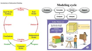
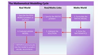
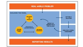
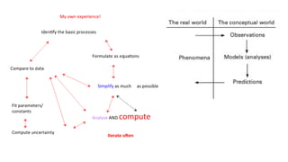
Introduction to Mathematical Modeling
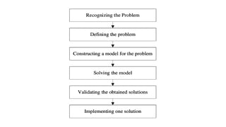
Modeling cycle
Introduction to Mathematical Modeling.  Optimization
Mathematical model
A mathematical model is a mathematical relation that describes some real-life
situations. Mathematical models are used to solve many real-life situations.
eg. launching a satellite, predicting the arrival of the monsoon, controlling
pollution due to vehicles
OR
Mathematical models are numerical or quantitative representations of a real-
world system. There are many different types of math models, and they common
involve constants and variables.
OR
A mathematical model is an abstract description of a concrete system using
mathematical concepts and language .
The process of developing a mathematical model is termed mathematical
modeling.
Introduction to Mathematical Modeling.  Optimization
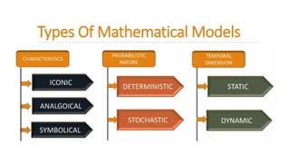
Types of Mathematical models
Mathematical models can be classified in a variety of ways, depending on their
structure,
Linear: The relationship between all variables in a model is linear, or
straightforward and sequential.
Nonlinear: The relationship between all variables in a model is not linear.
Static: The model does not consider time.
Dynamic: The model does consider changes over time.
Deterministic: A model with known variables.
Stochastic: A model with unknown variables.
Deductive: The model is based on theory.
Inductive: The model is based on observation or experience.
Floating: The model is neither deductive nor inductive.
What are different types of Mathematical Modelling?
Different types of math models includes:
• Static Vs Dynamic
• Linear Vs Nonlinear
• Explicit Vs Implicit
• Deterministic Vs Probabilistic (or stochastic)
• Discrete Vs Continuous
• Floating, Inductive, or Deductive
Objective function
• An objective function is a formula involving one or more decision variables,
denoted x1 , x 2 , … xn , that is to be optimized by determining the appropriate
values of those variables.
• It evaluates the accuracy of the model's output. The objective function is the
measure used to evaluate how well the model's output matches the desired
correct values.
• The objective function is a mathematical function that you want to optimize or
minimize/maximize in an optimization problem. It represents the goal you are
trying to achieve.
- In a typical optimization problem, you are looking to find the input variables
that either maximize or minimize the objective function.
- The objective function can be linear or nonlinear, convex or non-convex,
depending on the nature of the problem.
- Common types of objective functions include cost functions, profit functions,
utility functions etc.
The terminologies associated with Objective Function are as follows:
• Constraints: They are basically the conditional equations that govern the
Linear function
• Decision Variables: The variables whose values are to be found out. The
equations are solved so as to get the optimal value of these variables.
• Feasible Region: It is the region in the graph where the constraints are
satisfied and the decision variables are found at the corners of the region.
• Optimum Solution: The best possible solution that satisfies all constraints
and achieves the highest or lowest objective.
• Infeasible Solution: A solution that violates one or more constraints and
cannot be implemented or executed.
Constraints and Constraint surface
In mathematical modelling, a constraint is a condition or restriction
that limits the values of variables or the behaviour of a system.
Constraints can be represented mathematically using equations or
inequalities.
Types of constraints:
1. Equality constraints: Must be satisfied exactly (e.g., x + y = 10)
2. Inequality constraints: Must be satisfied within a range (e.g., x + y ≤ 10)
3. Boundary constraints: Limit the values of variables (e.g., 0 ≤ x ≤ 10)
4. Non-negativity constraints: Variables must be non-negative (e.g., x ≥ 0)
Constraint surfaces:
In two-dimensional space, a constraint can be represented as a line or curve.
In three-dimensional space, a constraint can be represented as a surface. A constraint surface is a
geometric representation of the constraint, showing the feasible region of solutions.
Example:
- A constraint like x + y = 10 can be represented as a line in 2D space.
- A constraint like x2
+ y2
≤ 10 can be represented as a circle in 2D space.
Constraint surfaces are useful in:
- Optimization problems: To find the maximum or minimum of a function subject to
constraints.
- Decision-making: To identify feasible solutions within the constraint boundaries.
- Modeling real-world systems: To account for physical or logical limitations.
Here are some examples of constraints and constraint surfaces in mathematical modeling:
Equality Constraint: x + y = 10
Constraint surface: A line in 2D space, where every point on the line satisfies the equation.
Inequality Constraint: x + y ≤ 10
Constraint surface: A half-plane in 2D space, where every point on one side of the line
satisfies the inequality.
Boundary Constraint: 0 ≤ x ≤ 10, 0 ≤ y ≤ 10
Constraint surface: A square in 2D space, where every point inside or on the boundary
satisfies the constraints.
Non-negativity Constraint: x ≥ 0, y ≥ 0
Constraint surface: A quadrant in 2D space, where every point in the quadrant satisfies the
constraints.
Circular Constraint: x2
+ y2
≤ 10
Constraint surface: A curved surface in 3D space, where every point on the surface satisfies the constraints.
Constraint surface: A circle in 2D space, where every point inside or on the circle satisfies the constraint.
Linear Programming:
Maximize: 2x + 3y
Subject to:
x + y ≤ 10
x ≥ 0, y ≥ 0
Constraint surface: A polygon in 2D space, where every point inside or on the boundary satisfies the
constraints.
Non-linear Programming:
Maximize: x2
+ y2
Subject to:
x + y ≤ 10
x ≥ 0, y ≥ 0
Constraint surface: A curved surface in 3D space, where every point on the surface satisfies the constraints.
Mathematical modeling characteristics and limitations
1.Simplification:
Mathematical models simplify complex real-world systems by focusing on
essential features.
Omitting minor details to focus on essential features.
Example: Modeling population growth using the logistic equation, ignoring
individual variations.
2. Abstraction:
Models abstract away irrelevant details to emphasize important relationships.
Representing complex systems using abstract concepts.
Example: Using differential equations to model electrical circuits, abstracting
away physical components.
3.Idealization:
Models often idealize or assume perfect conditions, like frictionless
surfaces.
Assuming perfect conditions, like frictionless surfaces.
Example: Modeling projectile motion, assuming no air resistance.
4. Mathematization:
Models translate real-world problems into mathematical language.
Example: Converting word problems into algebraic equations.
5 .Assumptions:
Models rely on assumptions, which may not always hold true.
Example: Assuming constant interest rates in financial modeling.
6.Approximations:
Models often use approximations, like linearizing nonlinear relationships.
Example: Using Taylor series expansions to approximate complex functions.
7. Uncertainty:
Models can be uncertain due to data limitations or inherent randomness.
Dealing with uncertainty due to data limitations or randomness.
Example: Using probability theory to model stock market fluctuations.
8. Scalability:
Models can be scaled up or down to represent different levels of complexity.
Scaling models up or down to represent different levels of complexity.
Example: Using the same model to simulate both individual and population-level
behavior.
9. Flexibility:
Models can be adapted or modified as new information becomes available.
Example: Updating weather forecasting models with new satellite data.
10. Validation:
Models must be validated against real-world data or observations.
Verifying models against real-world data or observations.
Example: Comparing climate model predictions with historical temperature record
11. Interpretability
Models should be interpretable and provide insights into the system.
Example: Using sensitivity analysis to understand how model outputs respond to input changes.
12. Predictive power:
Models aim to make accurate predictions or forecasts.
example: Using machine learning models to predict customer churn.
Formulating design problems in optimization techniques involves:
1. Defining the objective function: Identify the performance metric to optimize
(e.g., minimize cost, maximize efficiency).
2. Decision variables: Determine the design parameters to adjust (e.g., material
properties, geometric dimensions).
3. Constraints: Specify the limitations and requirements (e.g., physical laws,
manufacturing constraints).
4. Boundary conditions: Define the problem's scope and any fixed parameters.
5. Mathematical modeling: Represent the problem using mathematical
equations and relationships.
6. Optimization algorithm: Choose an appropriate optimization technique (e.g.,
linear programming, genetic algorithm).
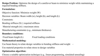
Design Problem: Optimize the design of a cantilever beam to minimize weight while maintaining a
required bending stiffness.
Formulation:
Objective function: Minimize weight (W)
Decision variables: Beam width (w), height (h), and length (L)
Constraints:
Bending stiffness (S) ≥ required stiffness
Material strength (σ) ≥ maximum stress
Manufacturing constraints (e.g., minimum thickness)-
Boundary conditions:
Fixed beam length (L) Fixed loading conditions
Mathematical modeling:
Use beam theory to relate design variables to bending stiffness and weight -
Use material properties to relate stress to design variables
Optimization algorithm:
Choose a suitable optimization technique (e.g., linear programming, simulated annealing)
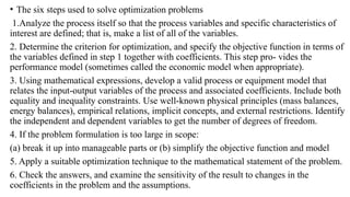
• The six steps used to solve optimization problems
1.Analyze the process itself so that the process variables and specific characteristics of
interest are defined; that is, make a list of all of the variables.
2. Determine the criterion for optimization, and specify the objective function in terms of
the variables defined in step 1 together with coefficients. This step pro- vides the
performance model (sometimes called the economic model when appropriate).
3. Using mathematical expressions, develop a valid process or equipment model that
relates the input-output variables of the process and associated coefficients. Include both
equality and inequality constraints. Use well-known physical principles (mass balances,
energy balances), empirical relations, implicit concepts, and external restrictions. Identify
the independent and dependent variables to get the number of degrees of freedom.
4. If the problem formulation is too large in scope:
(a) break it up into manageable parts or (b) simplify the objective function and model
5. Apply a suitable optimization technique to the mathematical statement of the problem.
6. Check the answers, and examine the sensitivity of the result to changes in the
coefficients in the problem and the assumptions.
Introduction to Mathematical Modeling.  Optimization

More Related Content

Introduction to Mathematical Modeling. Optimization

  • 1. A Study Material on Optimization Techniques (602213) (ME Design - Second Year ) by Mr. S D Martande
  • 2. Unit 1 Introduction to Mathematical Modeling • Introduction to Mathematical Modeling • Types of Modeling • Objective function • Constraints and Constraint surface • Mathematical modeling characteristics and limitations • Formulation of design problems
  • 3. History The beginnings of the subject operations research can be traced to the early period of World War II. During the war, the British military faced the problem of allocating very scarce and limited resources (such as fighter airplanes, radars, and submarines) to several activities (deployment to numerous targets and destinations). Because there were no systematic methods available to solve resource allocation problems, the military called upon a team of mathematicians to develop methods for solving the problem in a scientific manner. The methods developed by the team were instrumental in the winning of the Air Battle by Britain. These methods, such as linear programming, which were developed as a result of research on (military) operations, subsequently became known as the methods of operations research.
  • 4. Optimization Techniques • Optimization technique is a powerful tool to obtain the desired design parameters and best set of operating conditions . • Optimization concerns the minimization or maximization of functions. • It is used to solve complex design problems in order to improve cost, reliability, and performance in a wide range of applications. • Optimization is the process of obtaining the best result or benefit under a given set of circumstannces. • an act, process, or methodology of making something (such as a design, system, or decision) as fully perfect, functional, or effective as possible. • Optimization started its gradual perfection in mid-19th-century English, when it was derived from optimize, a word first used in the early part of that same century with the meaning "to make the best or most of." In basic applications, optimization refers to the act or process of making something as good as it can be.
  • 5. Engineering Optimization Techniques Examples • structural design (including pressure vessel design and welded beam design) • shape optimization. • topology optimization (including airfoils) • inverse optimization (a subset of the inverse problem) • processing planning. • product designs. • Product-Mix Problem • Use of Raw-Materials • Shipping Problems
  • 7. Introduction to Mathematical Modeling Modeling cycle
  • 11. Mathematical model A mathematical model is a mathematical relation that describes some real-life situations. Mathematical models are used to solve many real-life situations. eg. launching a satellite, predicting the arrival of the monsoon, controlling pollution due to vehicles OR Mathematical models are numerical or quantitative representations of a real- world system. There are many different types of math models, and they common involve constants and variables. OR A mathematical model is an abstract description of a concrete system using mathematical concepts and language . The process of developing a mathematical model is termed mathematical modeling.
  • 13. Types of Mathematical models Mathematical models can be classified in a variety of ways, depending on their structure, Linear: The relationship between all variables in a model is linear, or straightforward and sequential. Nonlinear: The relationship between all variables in a model is not linear. Static: The model does not consider time. Dynamic: The model does consider changes over time. Deterministic: A model with known variables. Stochastic: A model with unknown variables. Deductive: The model is based on theory. Inductive: The model is based on observation or experience. Floating: The model is neither deductive nor inductive.
  • 14. What are different types of Mathematical Modelling? Different types of math models includes: • Static Vs Dynamic • Linear Vs Nonlinear • Explicit Vs Implicit • Deterministic Vs Probabilistic (or stochastic) • Discrete Vs Continuous • Floating, Inductive, or Deductive
  • 15. Objective function • An objective function is a formula involving one or more decision variables, denoted x1 , x 2 , … xn , that is to be optimized by determining the appropriate values of those variables. • It evaluates the accuracy of the model's output. The objective function is the measure used to evaluate how well the model's output matches the desired correct values. • The objective function is a mathematical function that you want to optimize or minimize/maximize in an optimization problem. It represents the goal you are trying to achieve. - In a typical optimization problem, you are looking to find the input variables that either maximize or minimize the objective function. - The objective function can be linear or nonlinear, convex or non-convex, depending on the nature of the problem. - Common types of objective functions include cost functions, profit functions, utility functions etc.
  • 16. The terminologies associated with Objective Function are as follows: • Constraints: They are basically the conditional equations that govern the Linear function • Decision Variables: The variables whose values are to be found out. The equations are solved so as to get the optimal value of these variables. • Feasible Region: It is the region in the graph where the constraints are satisfied and the decision variables are found at the corners of the region. • Optimum Solution: The best possible solution that satisfies all constraints and achieves the highest or lowest objective. • Infeasible Solution: A solution that violates one or more constraints and cannot be implemented or executed.
  • 17. Constraints and Constraint surface In mathematical modelling, a constraint is a condition or restriction that limits the values of variables or the behaviour of a system. Constraints can be represented mathematically using equations or inequalities. Types of constraints: 1. Equality constraints: Must be satisfied exactly (e.g., x + y = 10) 2. Inequality constraints: Must be satisfied within a range (e.g., x + y ≤ 10) 3. Boundary constraints: Limit the values of variables (e.g., 0 ≤ x ≤ 10) 4. Non-negativity constraints: Variables must be non-negative (e.g., x ≥ 0)
  • 18. Constraint surfaces: In two-dimensional space, a constraint can be represented as a line or curve. In three-dimensional space, a constraint can be represented as a surface. A constraint surface is a geometric representation of the constraint, showing the feasible region of solutions. Example: - A constraint like x + y = 10 can be represented as a line in 2D space. - A constraint like x2 + y2 ≤ 10 can be represented as a circle in 2D space. Constraint surfaces are useful in: - Optimization problems: To find the maximum or minimum of a function subject to constraints. - Decision-making: To identify feasible solutions within the constraint boundaries. - Modeling real-world systems: To account for physical or logical limitations.
  • 19. Here are some examples of constraints and constraint surfaces in mathematical modeling: Equality Constraint: x + y = 10 Constraint surface: A line in 2D space, where every point on the line satisfies the equation. Inequality Constraint: x + y ≤ 10 Constraint surface: A half-plane in 2D space, where every point on one side of the line satisfies the inequality. Boundary Constraint: 0 ≤ x ≤ 10, 0 ≤ y ≤ 10 Constraint surface: A square in 2D space, where every point inside or on the boundary satisfies the constraints. Non-negativity Constraint: x ≥ 0, y ≥ 0 Constraint surface: A quadrant in 2D space, where every point in the quadrant satisfies the constraints.
  • 20. Circular Constraint: x2 + y2 ≤ 10 Constraint surface: A curved surface in 3D space, where every point on the surface satisfies the constraints. Constraint surface: A circle in 2D space, where every point inside or on the circle satisfies the constraint. Linear Programming: Maximize: 2x + 3y Subject to: x + y ≤ 10 x ≥ 0, y ≥ 0 Constraint surface: A polygon in 2D space, where every point inside or on the boundary satisfies the constraints. Non-linear Programming: Maximize: x2 + y2 Subject to: x + y ≤ 10 x ≥ 0, y ≥ 0 Constraint surface: A curved surface in 3D space, where every point on the surface satisfies the constraints.
  • 21. Mathematical modeling characteristics and limitations 1.Simplification: Mathematical models simplify complex real-world systems by focusing on essential features. Omitting minor details to focus on essential features. Example: Modeling population growth using the logistic equation, ignoring individual variations. 2. Abstraction: Models abstract away irrelevant details to emphasize important relationships. Representing complex systems using abstract concepts. Example: Using differential equations to model electrical circuits, abstracting away physical components.
  • 22. 3.Idealization: Models often idealize or assume perfect conditions, like frictionless surfaces. Assuming perfect conditions, like frictionless surfaces. Example: Modeling projectile motion, assuming no air resistance. 4. Mathematization: Models translate real-world problems into mathematical language. Example: Converting word problems into algebraic equations. 5 .Assumptions: Models rely on assumptions, which may not always hold true. Example: Assuming constant interest rates in financial modeling.
  • 23. 6.Approximations: Models often use approximations, like linearizing nonlinear relationships. Example: Using Taylor series expansions to approximate complex functions. 7. Uncertainty: Models can be uncertain due to data limitations or inherent randomness. Dealing with uncertainty due to data limitations or randomness. Example: Using probability theory to model stock market fluctuations. 8. Scalability: Models can be scaled up or down to represent different levels of complexity. Scaling models up or down to represent different levels of complexity. Example: Using the same model to simulate both individual and population-level behavior.
  • 24. 9. Flexibility: Models can be adapted or modified as new information becomes available. Example: Updating weather forecasting models with new satellite data. 10. Validation: Models must be validated against real-world data or observations. Verifying models against real-world data or observations. Example: Comparing climate model predictions with historical temperature record 11. Interpretability Models should be interpretable and provide insights into the system. Example: Using sensitivity analysis to understand how model outputs respond to input changes. 12. Predictive power: Models aim to make accurate predictions or forecasts. example: Using machine learning models to predict customer churn.
  • 25. Formulating design problems in optimization techniques involves: 1. Defining the objective function: Identify the performance metric to optimize (e.g., minimize cost, maximize efficiency). 2. Decision variables: Determine the design parameters to adjust (e.g., material properties, geometric dimensions). 3. Constraints: Specify the limitations and requirements (e.g., physical laws, manufacturing constraints). 4. Boundary conditions: Define the problem's scope and any fixed parameters. 5. Mathematical modeling: Represent the problem using mathematical equations and relationships. 6. Optimization algorithm: Choose an appropriate optimization technique (e.g., linear programming, genetic algorithm).
  • 26. Design Problem: Optimize the design of a cantilever beam to minimize weight while maintaining a required bending stiffness. Formulation: Objective function: Minimize weight (W) Decision variables: Beam width (w), height (h), and length (L) Constraints: Bending stiffness (S) ≥ required stiffness Material strength (σ) ≥ maximum stress Manufacturing constraints (e.g., minimum thickness)- Boundary conditions: Fixed beam length (L) Fixed loading conditions Mathematical modeling: Use beam theory to relate design variables to bending stiffness and weight - Use material properties to relate stress to design variables Optimization algorithm: Choose a suitable optimization technique (e.g., linear programming, simulated annealing)
  • 27. • The six steps used to solve optimization problems 1.Analyze the process itself so that the process variables and specific characteristics of interest are defined; that is, make a list of all of the variables. 2. Determine the criterion for optimization, and specify the objective function in terms of the variables defined in step 1 together with coefficients. This step pro- vides the performance model (sometimes called the economic model when appropriate). 3. Using mathematical expressions, develop a valid process or equipment model that relates the input-output variables of the process and associated coefficients. Include both equality and inequality constraints. Use well-known physical principles (mass balances, energy balances), empirical relations, implicit concepts, and external restrictions. Identify the independent and dependent variables to get the number of degrees of freedom. 4. If the problem formulation is too large in scope: (a) break it up into manageable parts or (b) simplify the objective function and model 5. Apply a suitable optimization technique to the mathematical statement of the problem. 6. Check the answers, and examine the sensitivity of the result to changes in the coefficients in the problem and the assumptions.