際際滷

際際滷Share a Scribd company logo
Bayesian Learning
Na?ve Bayes Classification
? Naive Bayes is among one of the most simple and powerful algorithms
for classification based on Bayes¨ Theorem with an assumption of
independence among predictors.
? Naive Bayes model is easy to build and particularly useful for very large
data sets. There are two parts to this algorithm:
1. Naive
2. Bayes
? The Naive Bayes classifier assumes that the presence of a feature in a
class is unrelated to any other feature. The Algorithm is `naive¨ because
it makes assumptions that may or may not turn out to be correct.
Contd..
? Naive Bayes model is easy to build and particularly useful for very
large data sets.
? Along with simplicity, Naive Bayes is known to outperform even highly
sophisticated classification methods.
Prerequisites for Bayes Theorem
Experiment
? An experiment is defined as the planned operation carried out under controlled
condition such as tossing a coin, drawing a card and rolling a dice, etc.
Sample Space
? During an experiment what we get as a result is called as possible outcomes and
the set of all possible outcome of an event is known as sample space. For
example, if we are rolling a dice, sample space will be:
S1 = {1, 2, 3, 4, 5, 6}
Similarly, if our experiment is related to toss a coin and recording its outcomes,
then sample space will be:
S2 = {Head, Tail}
Prerequisites for Bayes Theorem
Event
? Event is defined as subset of sample space in an experiment. Further, it is also
called as set of outcomes
? Assume in our experiment of rolling a dice, there are two event A and B such
that;
? A = Event when an even number is obtained = {2, 4, 6}
? B = Event when a number is greater than 4 = {5, 6}
? Probability of the event A ''P(A)''= Number of favourable outcomes / Total
number of possible outcomes
P(E) = 3/6 =1/2 =0.5
? Similarly, Probability of the event B ''P(B)''= Number of favourable outcomes /
Total number of possible outcomes
=2/6 =1/3 =0.333
? Union of event A and B:
A B = {2, 4, 5, 6}
“
P(A B)=P(A)+P(B)-P(A
“ ”B)
Prerequisites for Bayes Theorem
Event
? Intersection of event A and B: A”B= {6}
When A and B are independent events, the probability of A
intersection B, P(A B) = P(A)〜P(B).
?
? Disjoint Event: If the intersection of the event A and B
is an empty set or null then such events are known
as disjoint event or mutually exclusive events also.
Prerequisites for Bayes Theorem
Exhaustive Event:
? As per the name suggests, a set of events where at least one event occurs at a time, called exhaustive event of an
experiment.
? Thus, two events A and B are said to be exhaustive if either A or B definitely occur at a time and both are mutually
exclusive for e.g., while tossing a coin, either it will be a Head or may be a Tail.
Independent Event:
? Two events are said to be independent when occurrence of one event does not affect the occurrence of another
event. In simple words we can say that the probability of outcome of both events does not depends one another.
? Mathematically, two events A and B are said to be independent if:
? P(A ” B) = P(AB) = P(A)*P(B)
Conditional Probability:
? Conditional probability is defined as the probability of an event A, given that another event B has already
occurred (i.e. A conditional B). This is represented by P(A|B) and we can define it as:
? P(A|B) = P(A ” B) / P(B)
Prerequisites for Bayes Theorem
Law of Total Probability
? For two events A and B associated with a sample space S, the sample space can be divided into a
set A ” B , A ” B, A ” B, A ” B . This set is said to be mutually disjoint or pairwise disjoint because
> > > >
any pair of sets in it is disjoint. Elements of this set are better known as a partition of sample
space.
Prerequisites for Bayes Theorem
? Law of Total Probability Statement
? Let events C1, C2 . . . Cn form partitions of the sample space S, where all the events
have a non-zero probability of occurrence. For any event, A associated with S,
according to the total probability theorem,
? P(A) = P(C1)P(A| C1) + P(C2)P(A|C2) + P(C3)P(A| C3) + . . . . . + P(Cn)P(A| Cn)
? Hence, the theorem can be stated in form of equation as,
? If we put a naive assumption to the Bayes¨ theorem, which is,
independence among the features. So now, we split evidence into the
independent parts.
? Now, if any two events A and B are independent, then,
P(A,B) = P(A)P(B)
Hence, we reach to the result:
which can be expressed as:
Prediction using Bayes Theorem - Example
The dataset is divided into two parts,
namely, feature matrix and the
response vector.
?Feature matrix contains all the
vectors(rows) of dataset in which each
vector consists of the value of
dependent features. In above dataset,
features are `Outlook¨, `Temperature¨,
`Humidity¨ and `Windy¨.
?Response vector contains the value of
class variable(prediction or output) for
each row of feature matrix. In above
dataset, the class variable name is `Play
golf¨.
Example contd..
We need to find P(xi | yj) for each xi in X and yj in y. All these calculations have been demonstrated in the
tables below:
We have calculated P(xi | yj) for each xi in X and yj in y
manually in the tables 1-4. For example, probability of playing
golf given that the temperature is cool, i.e
P(temp = cool | play golf = Yes) = 3/9.
Also, we need to find class probabilities (P(y)) which has been
calculated in the table 5. For example, P(play golf = Yes) =
9/14.
So now, we are done with our pre-computations and the
classifier is ready!
? Let us test it on a new set of features (let us call it today):
? today = (Sunny, Hot, Normal, False)
? So, probability of playing golf is given by:
? and probability to not play golf is given by:
? Since, P(today) is common in both probabilities, we can ignore P(today) and
find proportional probabilities as:
and
Test C Rainy, Mild, High, False
? Now, since
? These numbers can be converted into a probability by making the sum
equal to 1 (normalization):
And
Since
So, prediction that golf would be played is `Yes¨.
Introduction to Naive bayes and baysian belief network
Advantages of Na?ve Bayes
? It is not only a simple approach but also a fast and accurate method for
prediction.
? Naive Bayes has very low computation cost.
? It can efficiently work on a large dataset.
? It performs well in case of discrete response variable compared to the
continuous variable.
? It can be used with multiple class prediction problems.
? It also performs well in the case of text analytics problems.
? When the assumption of independence holds, a Naive Bayes classifier
performs better compared to other models like logistic regression.
Disadvantages
? The assumption of independent features. In practice, it is almost
impossible that model will get a set of predictors which are entirely
independent.
? If there is no training tuple of a particular class, this causes zero
posterior probability. In this case, the model is unable to make
predictions. This problem is known as Zero Probability/Frequency
Problem.
Applications
? Real time Prediction: Naive Bayes is an eager learning classifier and it is sure fast. Thus, it
could be used for making predictions in real time.
? Multi class Prediction: This algorithm is also well known for multi class prediction feature.
Here we can predict the probability of multiple classes of target variable.
? Text classification/ Spam Filtering/ Sentiment Analysis: Naive Bayes classifiers are mostly
used in text classification. Due to better result in multi class problems and independence
rule it has higher success rate as compared to other algorithms. As a result, it is widely
used in Spam filtering (identify spam e-mail) and Sentiment Analysis (in social media
analysis, to identify positive and negative customer sentiments)
? Recommendation System: Naive Bayes Classifier and Collaborative Filtering together
builds a Recommendation System that uses machine learning and data mining techniques
to filter unseen information and predict whether a user would like a given resource or not
Zero Probability Problem in Na?ve Bayes Classifier
Introduction to Naive bayes and baysian belief network
Bayesian Belief Network
? "A Bayesian network is a probabilistic graphical model which
represents a set of variables and their conditional dependencies using
a directed acyclic graph."
? It is also called a Bayes network, belief network, decision network,
or Bayesian model.
? Bayesian networks are probabilistic, because these networks are built
from a probability distribution, and also use probability theory for
prediction and anomaly detection.
? Real world applications are probabilistic in nature, and to represent
the relationship between multiple events, we need a Bayesian
network.
? It can also be used in various tasks including prediction, anomaly
detection, diagnostics, automated insight, reasoning, time series
prediction, and decision making under uncertainty.
? Bayesian Network can be used for building models from data and
experts opinions, and it consists of two parts:
? Directed Acyclic Graph
? Conditional Probabilities Table (CPT).
Bayesian Belief Network
? A Bayesian network graph is made up of nodes and Arcs
(directed links), where:
? Each node corresponds to the random variables, and a variable
can be continuous or discrete.
? Arc or directed arrows represent the causal relationship or
conditional probabilities between random variables. These
directed links or arrows connect the pair of nodes in the graph.
These links represent that one node directly influence the
other node, and if there is no directed link that means that
nodes are independent with each other
? In the diagram, A, B, C, and D are random variables represented by
the nodes of the network graph.
? If we are considering node B, which is connected with node A by a
directed arrow, then node A is called the parent of Node B.
? Node C is conditionally independent of node A.
Bayesian Belief Network
? Each node in the Bayesian network has condition probability
distribution P(Xi |Parent(Xi) ), which determines the effect of the
parent on that node.
? Bayesian network is based on Joint probability distribution and
conditional probability.
Bayesian Belief Network
31
Bayesian Belief Networks (BNs)
? Definition: BN = (DAG, CPD)
C DAG: directed acyclic graph (BN¨s structure)
? Nodes: random variables (typically binary or discrete,
but methods also exist to handle continuous variables)
? Arcs: indicate probabilistic dependencies between nodes
(lack of link signifies conditional independence)
C CPD: conditional probability distribution (BN¨s parameters)
? Conditional probabilities at each node, usually stored as a table
(conditional probability table, or CPT)
C Root nodes are a special case C no parents, so just use priors
in CPD:
32
Example BN
a
b c
d e
P(C|A) = 0.2
P(C|?A) = 0.005
P(B|A) = 0.3
P(B|?A) = 0.001
P(A) = 0.001
P(D|B,C) = 0.1
P(D|B,?C) = 0.01
P(D|?B,C) = 0.01
P(D|?B,?C) = 0.00001
P(E|C) = 0.4
P(E|?C) =
0.002
Note that we only specify P(A) etc., not P(?A), since they have to add to
one
33
? Conditional independence assumption
C
where q is any set of variables
(nodes) other than and its successors
C blocks influence of other nodes on
and its successors (q influences only
through variables in )
C With this assumption, the complete joint probability distribution of all
variables in the network can be represented by (recovered from) local
CPDs by chaining these CPDs:
q
Conditional independence and chaining
34
Chaining: Example
Computing the joint probability for all variables is easy:
P(a, b, c, d, e)
= P(e | a, b, c, d) P(a, b, c, d) by the product rule
= P(e | c) P(a, b, c, d) by cond. indep.
assumption
= P(e | c) P(d | a, b, c) P(a, b, c)
= P(e | c) P(d | b, c) P(c | a, b) P(a, b)
= P(e | c) P(d | b, c) P(c | a) P(b | a) P(a)
a
b c
d e
35
A B C
Conditional
Independence
The joint probability is: P(A,B,C)= P(A)*P(B)*P(C)
A
B C The joint probability is: P(A,B,C)= P(B | A)*P(C|A)*P(A)
C
A B
Causal
Independence The joint probability is: P(A,B,C)= P(C |A, B)*P(A)*P(B)
B
A C
Markov
Independence
The joint probability is: P(A,B,C)= P(C |B)*P(B|A)*P(A)
Marginal
Independence
Example
? Example: Harry installed a new burglar alarm at his home to detect burglary.
The alarm reliably responds at detecting a burglary but also responds for minor
earthquakes. Harry has two neighbours David and Sophia, who have taken a
responsibility to inform Harry at work when they hear the alarm. David always
calls Harry when he hears the alarm, but sometimes he got confused with the
phone ringing and calls at that time too. On the other hand, Sophia likes to listen
to high music, so sometimes she misses to hear the alarm. Here we would like to
compute the probability of Burglary Alarm.
? Problem:
? Calculate the probability that alarm has sounded, but there is neither a
burglary, nor an earthquake occurred, and David and Sophia both called
the Harry.
36
37
.001
.31
? We can write the events of problem statement in the form of
probability: P[D, S, A, B, E], can rewrite the above
probability statement using joint probability distribution:
P[D, S, A, B, E]= P[D | S, A, B, E]. P[S, A, B, E]
=P[D | S, A, B, E]. P[S | A, B, E]. P[A, B, E]
= P [D| A]. P [ S| A, B, E]. P[ A, B, E]
= P[D | A]. P[ S | A]. P[A| B, E]. P[B, E]
= P[D | A ]. P[S | A]. P[A| B, E]. P[B]. P[E]
Calculate the probability that alarm has sounded, but there
is neither a burglary, nor an earthquake occurred, and
David and Sophia both called the Harry.
P(S, D, A, ?B, ?E) = P (S|A) *P (D|A)*P (A|?B,
?E) *P (?B) *P (?E).
= 0.75* 0.91* 0.001* 0.998*0.999
= 0.00068045
38
39
Maximum A Posteriori (MAP)
Hypothesis and Maximum Likelihood
? Goal: To find the most probable hypothesis h from a set of
candidate hypotheses H given the observed data D.
? MAP Hypothesis, hMAP = argmax h H
( P(h|D)
= argmax h H
( P(D|h)P(h)/P(D)
= argmax h H
( P(D|h)P(h)
? If every hypothesis in H is equally probable a priori, we only
need to consider the likelihood of the data D given h, P(D|
h). Then, hMAP becomes the Maximum Likelihood,
hML= argmax h H
( P(D|h)
THANK YOU

More Related Content

Similar to Introduction to Naive bayes and baysian belief network (20)

PDF
Warmup_New.pdf
HongAnhNguyn285885
?
PPTX
Artificial Intelligence Notes Unit 3
DigiGurukul
?
PPTX
Supervised models
Hasan Badran
?
PDF
naive bayes example.pdf
SingamalaBalaji
?
PDF
naive bayes example.pdf
SingamalaBalaji
?
PDF
Data classification sammer
Sammer Qader
?
PPTX
Na?ve Bayes Classifier Algorithm.pptx
Shubham Jaybhaye
?
PDF
19BayesTheoremClassification19BayesTheoremClassification.ppt
Nishant83346
?
PPTX
Applications of Classification Algorithm.pptx
nagarajan740445
?
PPT
Uncertainty
Digvijay Singh
?
PDF
Na?ve Bayes Machine Learning Classification with R Programming: A case study ...
SubmissionResearchpa
?
PPTX
Na?ve Bayes Classifier Algorithm.pptx
PriyadharshiniG41
?
PPTX
artificial intelligence and uncertain reasoning
johngeorgakis99
?
PPTX
Bayes' theorem
Dr. C.V. Suresh Babu
?
PPT
NaiveBayes.ppt Naive Bayes algorithm machine learning
AmgadAbdallah2
?
PPT
NaiveBayes.ppt
CristopherAbalorio2
?
PPT
NaiveBayes.ppt
sabbirice08
?
PPT
NaiveBayes.ppt
EslamAbdAlAziz4
?
PPTX
Data Analytics with Data Science Algorithm
kumari36
?
PDF
Sample Space and Event,Probability,The Axioms of Probability,Bayes Theorem
Bharath kumar Karanam
?
Warmup_New.pdf
HongAnhNguyn285885
?
Artificial Intelligence Notes Unit 3
DigiGurukul
?
Supervised models
Hasan Badran
?
naive bayes example.pdf
SingamalaBalaji
?
naive bayes example.pdf
SingamalaBalaji
?
Data classification sammer
Sammer Qader
?
Na?ve Bayes Classifier Algorithm.pptx
Shubham Jaybhaye
?
19BayesTheoremClassification19BayesTheoremClassification.ppt
Nishant83346
?
Applications of Classification Algorithm.pptx
nagarajan740445
?
Uncertainty
Digvijay Singh
?
Na?ve Bayes Machine Learning Classification with R Programming: A case study ...
SubmissionResearchpa
?
Na?ve Bayes Classifier Algorithm.pptx
PriyadharshiniG41
?
artificial intelligence and uncertain reasoning
johngeorgakis99
?
Bayes' theorem
Dr. C.V. Suresh Babu
?
NaiveBayes.ppt Naive Bayes algorithm machine learning
AmgadAbdallah2
?
NaiveBayes.ppt
CristopherAbalorio2
?
NaiveBayes.ppt
sabbirice08
?
NaiveBayes.ppt
EslamAbdAlAziz4
?
Data Analytics with Data Science Algorithm
kumari36
?
Sample Space and Event,Probability,The Axioms of Probability,Bayes Theorem
Bharath kumar Karanam
?

Recently uploaded (20)

PPTX
CST413 KTU S7 CSE Machine Learning Neural Networks and Support Vector Machine...
resming1
?
PDF
Rapid Prototyping for XR: Lecture 3 - Video and Paper Prototyping
Mark Billinghurst
?
PDF
13th International Conference of Security, Privacy and Trust Management (SPTM...
ijcisjournal
?
PPT
????? ???? ????? ??? ?? ???? ??? ???????
???? ??? ?????
?
PPTX
CST413 KTU S7 CSE Machine Learning Introduction Parameter Estimation MLE MAP ...
resming1
?
PDF
NFPA 10 - Estandar para extintores de incendios portatiles (ed.22 ENG).pdf
Oscar Orozco
?
PPTX
Work at Height training for workers .pptx
cecos12
?
PPTX
Tesla-Stock-Analysis-and-Forecast.pptx (1).pptx
moonsony54
?
PPTX
Functions in Python Programming Language
BeulahS2
?
PDF
May 2025: Top 10 Read Articles in Data Mining & Knowledge Management Process
IJDKP
?
PDF
Generative AI & Scientific Research : Catalyst for Innovation, Ethics & Impact
AlqualsaDIResearchGr
?
PDF
How to Buy Verified CashApp Accounts IN 2025
Buy Verified CashApp Accounts
?
PPTX
Introduction to Python Programming Language
merlinjohnsy
?
PPSX
OOPS Concepts in Python and Exception Handling
Dr. A. B. Shinde
?
PDF
i氏Y創_Miipher and Miipher2 .
鰻粥京晦粥皆幄塀氏芙
?
PDF
lesson4-occupationalsafetyandhealthohsstandards-240812020130-1a7246d0.pdf
arvingallosa3
?
PDF
Plant Control_EST_85520-01_en_AllChanges_20220127.pdf
DarshanaChathuranga4
?
PDF
Rapid Prototyping for XR: Lecture 1 Introduction to Prototyping
Mark Billinghurst
?
PPTX
Stability of IBR Dominated Grids - IEEE PEDG 2025 - short.pptx
ssuser307730
?
PDF
01-introduction to the ProcessDesign.pdf
StiveBrack
?
CST413 KTU S7 CSE Machine Learning Neural Networks and Support Vector Machine...
resming1
?
Rapid Prototyping for XR: Lecture 3 - Video and Paper Prototyping
Mark Billinghurst
?
13th International Conference of Security, Privacy and Trust Management (SPTM...
ijcisjournal
?
????? ???? ????? ??? ?? ???? ??? ???????
???? ??? ?????
?
CST413 KTU S7 CSE Machine Learning Introduction Parameter Estimation MLE MAP ...
resming1
?
NFPA 10 - Estandar para extintores de incendios portatiles (ed.22 ENG).pdf
Oscar Orozco
?
Work at Height training for workers .pptx
cecos12
?
Tesla-Stock-Analysis-and-Forecast.pptx (1).pptx
moonsony54
?
Functions in Python Programming Language
BeulahS2
?
May 2025: Top 10 Read Articles in Data Mining & Knowledge Management Process
IJDKP
?
Generative AI & Scientific Research : Catalyst for Innovation, Ethics & Impact
AlqualsaDIResearchGr
?
How to Buy Verified CashApp Accounts IN 2025
Buy Verified CashApp Accounts
?
Introduction to Python Programming Language
merlinjohnsy
?
OOPS Concepts in Python and Exception Handling
Dr. A. B. Shinde
?
i氏Y創_Miipher and Miipher2 .
鰻粥京晦粥皆幄塀氏芙
?
lesson4-occupationalsafetyandhealthohsstandards-240812020130-1a7246d0.pdf
arvingallosa3
?
Plant Control_EST_85520-01_en_AllChanges_20220127.pdf
DarshanaChathuranga4
?
Rapid Prototyping for XR: Lecture 1 Introduction to Prototyping
Mark Billinghurst
?
Stability of IBR Dominated Grids - IEEE PEDG 2025 - short.pptx
ssuser307730
?
01-introduction to the ProcessDesign.pdf
StiveBrack
?
Ad

Introduction to Naive bayes and baysian belief network

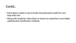
  • 2. Na?ve Bayes Classification ? Naive Bayes is among one of the most simple and powerful algorithms for classification based on Bayes¨ Theorem with an assumption of independence among predictors. ? Naive Bayes model is easy to build and particularly useful for very large data sets. There are two parts to this algorithm: 1. Naive 2. Bayes ? The Naive Bayes classifier assumes that the presence of a feature in a class is unrelated to any other feature. The Algorithm is `naive¨ because it makes assumptions that may or may not turn out to be correct.
  • 3. Contd.. ? Naive Bayes model is easy to build and particularly useful for very large data sets. ? Along with simplicity, Naive Bayes is known to outperform even highly sophisticated classification methods.
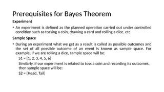
  • 4. Prerequisites for Bayes Theorem Experiment ? An experiment is defined as the planned operation carried out under controlled condition such as tossing a coin, drawing a card and rolling a dice, etc. Sample Space ? During an experiment what we get as a result is called as possible outcomes and the set of all possible outcome of an event is known as sample space. For example, if we are rolling a dice, sample space will be: S1 = {1, 2, 3, 4, 5, 6} Similarly, if our experiment is related to toss a coin and recording its outcomes, then sample space will be: S2 = {Head, Tail}
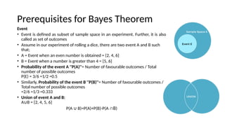
  • 5. Prerequisites for Bayes Theorem Event ? Event is defined as subset of sample space in an experiment. Further, it is also called as set of outcomes ? Assume in our experiment of rolling a dice, there are two event A and B such that; ? A = Event when an even number is obtained = {2, 4, 6} ? B = Event when a number is greater than 4 = {5, 6} ? Probability of the event A ''P(A)''= Number of favourable outcomes / Total number of possible outcomes P(E) = 3/6 =1/2 =0.5 ? Similarly, Probability of the event B ''P(B)''= Number of favourable outcomes / Total number of possible outcomes =2/6 =1/3 =0.333 ? Union of event A and B: A B = {2, 4, 5, 6} “ P(A B)=P(A)+P(B)-P(A “ ”B)
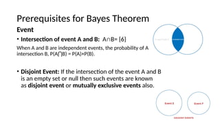
  • 6. Prerequisites for Bayes Theorem Event ? Intersection of event A and B: A”B= {6} When A and B are independent events, the probability of A intersection B, P(A B) = P(A)〜P(B). ? ? Disjoint Event: If the intersection of the event A and B is an empty set or null then such events are known as disjoint event or mutually exclusive events also.
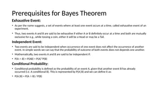
  • 7. Prerequisites for Bayes Theorem Exhaustive Event: ? As per the name suggests, a set of events where at least one event occurs at a time, called exhaustive event of an experiment. ? Thus, two events A and B are said to be exhaustive if either A or B definitely occur at a time and both are mutually exclusive for e.g., while tossing a coin, either it will be a Head or may be a Tail. Independent Event: ? Two events are said to be independent when occurrence of one event does not affect the occurrence of another event. In simple words we can say that the probability of outcome of both events does not depends one another. ? Mathematically, two events A and B are said to be independent if: ? P(A ” B) = P(AB) = P(A)*P(B) Conditional Probability: ? Conditional probability is defined as the probability of an event A, given that another event B has already occurred (i.e. A conditional B). This is represented by P(A|B) and we can define it as: ? P(A|B) = P(A ” B) / P(B)
  • 8. Prerequisites for Bayes Theorem Exhaustive Event: ? As per the name suggests, a set of events where at least one event occurs at a time, called exhaustive event of an experiment. ? Thus, two events A and B are said to be exhaustive if either A or B definitely occur at a time and both are mutually exclusive for e.g., while tossing a coin, either it will be a Head or may be a Tail. Independent Event: ? Two events are said to be independent when occurrence of one event does not affect the occurrence of another event. In simple words we can say that the probability of outcome of both events does not depends one another. ? Mathematically, two events A and B are said to be independent if: ? P(A ” B) = P(AB) = P(A)*P(B) Conditional Probability: ? Conditional probability is defined as the probability of an event A, given that another event B has already occurred (i.e. A conditional B). This is represented by P(A|B) and we can define it as: ? P(A|B) = P(A ” B) / P(B)
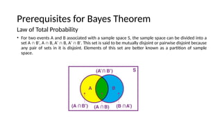
  • 9. Prerequisites for Bayes Theorem Law of Total Probability ? For two events A and B associated with a sample space S, the sample space can be divided into a set A ” B , A ” B, A ” B, A ” B . This set is said to be mutually disjoint or pairwise disjoint because > > > > any pair of sets in it is disjoint. Elements of this set are better known as a partition of sample space.
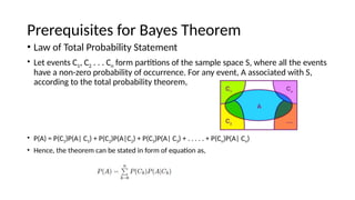
  • 10. Prerequisites for Bayes Theorem ? Law of Total Probability Statement ? Let events C1, C2 . . . Cn form partitions of the sample space S, where all the events have a non-zero probability of occurrence. For any event, A associated with S, according to the total probability theorem, ? P(A) = P(C1)P(A| C1) + P(C2)P(A|C2) + P(C3)P(A| C3) + . . . . . + P(Cn)P(A| Cn) ? Hence, the theorem can be stated in form of equation as,
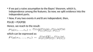
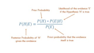
  • 11. ? If we put a naive assumption to the Bayes¨ theorem, which is, independence among the features. So now, we split evidence into the independent parts. ? Now, if any two events A and B are independent, then, P(A,B) = P(A)P(B) Hence, we reach to the result: which can be expressed as:
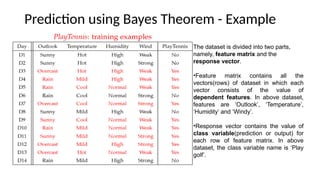
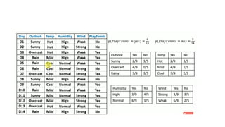
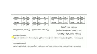
  • 12. Prediction using Bayes Theorem - Example The dataset is divided into two parts, namely, feature matrix and the response vector. ?Feature matrix contains all the vectors(rows) of dataset in which each vector consists of the value of dependent features. In above dataset, features are `Outlook¨, `Temperature¨, `Humidity¨ and `Windy¨. ?Response vector contains the value of class variable(prediction or output) for each row of feature matrix. In above dataset, the class variable name is `Play golf¨.
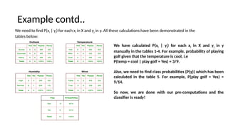
  • 13. Example contd.. We need to find P(xi | yj) for each xi in X and yj in y. All these calculations have been demonstrated in the tables below: We have calculated P(xi | yj) for each xi in X and yj in y manually in the tables 1-4. For example, probability of playing golf given that the temperature is cool, i.e P(temp = cool | play golf = Yes) = 3/9. Also, we need to find class probabilities (P(y)) which has been calculated in the table 5. For example, P(play golf = Yes) = 9/14. So now, we are done with our pre-computations and the classifier is ready!
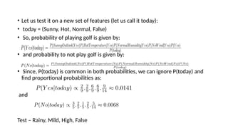
  • 14. ? Let us test it on a new set of features (let us call it today): ? today = (Sunny, Hot, Normal, False) ? So, probability of playing golf is given by: ? and probability to not play golf is given by: ? Since, P(today) is common in both probabilities, we can ignore P(today) and find proportional probabilities as: and Test C Rainy, Mild, High, False
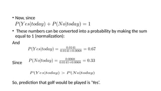
  • 15. ? Now, since ? These numbers can be converted into a probability by making the sum equal to 1 (normalization): And Since So, prediction that golf would be played is `Yes¨.
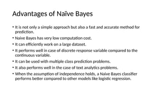
  • 18. Advantages of Na?ve Bayes ? It is not only a simple approach but also a fast and accurate method for prediction. ? Naive Bayes has very low computation cost. ? It can efficiently work on a large dataset. ? It performs well in case of discrete response variable compared to the continuous variable. ? It can be used with multiple class prediction problems. ? It also performs well in the case of text analytics problems. ? When the assumption of independence holds, a Naive Bayes classifier performs better compared to other models like logistic regression.
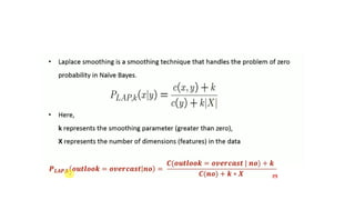
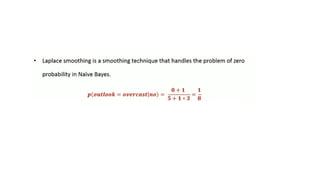
  • 19. Disadvantages ? The assumption of independent features. In practice, it is almost impossible that model will get a set of predictors which are entirely independent. ? If there is no training tuple of a particular class, this causes zero posterior probability. In this case, the model is unable to make predictions. This problem is known as Zero Probability/Frequency Problem.
  • 20. Applications ? Real time Prediction: Naive Bayes is an eager learning classifier and it is sure fast. Thus, it could be used for making predictions in real time. ? Multi class Prediction: This algorithm is also well known for multi class prediction feature. Here we can predict the probability of multiple classes of target variable. ? Text classification/ Spam Filtering/ Sentiment Analysis: Naive Bayes classifiers are mostly used in text classification. Due to better result in multi class problems and independence rule it has higher success rate as compared to other algorithms. As a result, it is widely used in Spam filtering (identify spam e-mail) and Sentiment Analysis (in social media analysis, to identify positive and negative customer sentiments) ? Recommendation System: Naive Bayes Classifier and Collaborative Filtering together builds a Recommendation System that uses machine learning and data mining techniques to filter unseen information and predict whether a user would like a given resource or not
  • 21. Zero Probability Problem in Na?ve Bayes Classifier
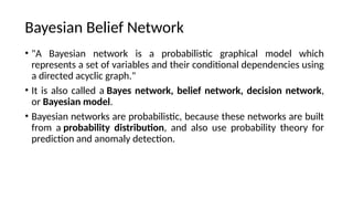
  • 26. Bayesian Belief Network ? "A Bayesian network is a probabilistic graphical model which represents a set of variables and their conditional dependencies using a directed acyclic graph." ? It is also called a Bayes network, belief network, decision network, or Bayesian model. ? Bayesian networks are probabilistic, because these networks are built from a probability distribution, and also use probability theory for prediction and anomaly detection.
  • 27. ? Real world applications are probabilistic in nature, and to represent the relationship between multiple events, we need a Bayesian network. ? It can also be used in various tasks including prediction, anomaly detection, diagnostics, automated insight, reasoning, time series prediction, and decision making under uncertainty. ? Bayesian Network can be used for building models from data and experts opinions, and it consists of two parts: ? Directed Acyclic Graph ? Conditional Probabilities Table (CPT). Bayesian Belief Network
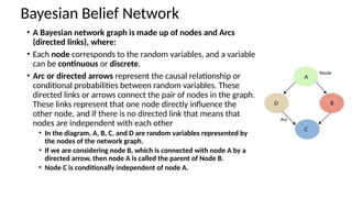
  • 28. ? A Bayesian network graph is made up of nodes and Arcs (directed links), where: ? Each node corresponds to the random variables, and a variable can be continuous or discrete. ? Arc or directed arrows represent the causal relationship or conditional probabilities between random variables. These directed links or arrows connect the pair of nodes in the graph. These links represent that one node directly influence the other node, and if there is no directed link that means that nodes are independent with each other ? In the diagram, A, B, C, and D are random variables represented by the nodes of the network graph. ? If we are considering node B, which is connected with node A by a directed arrow, then node A is called the parent of Node B. ? Node C is conditionally independent of node A. Bayesian Belief Network
  • 30. ? Each node in the Bayesian network has condition probability distribution P(Xi |Parent(Xi) ), which determines the effect of the parent on that node. ? Bayesian network is based on Joint probability distribution and conditional probability. Bayesian Belief Network
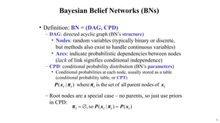
  • 31. 31 Bayesian Belief Networks (BNs) ? Definition: BN = (DAG, CPD) C DAG: directed acyclic graph (BN¨s structure) ? Nodes: random variables (typically binary or discrete, but methods also exist to handle continuous variables) ? Arcs: indicate probabilistic dependencies between nodes (lack of link signifies conditional independence) C CPD: conditional probability distribution (BN¨s parameters) ? Conditional probabilities at each node, usually stored as a table (conditional probability table, or CPT) C Root nodes are a special case C no parents, so just use priors in CPD:
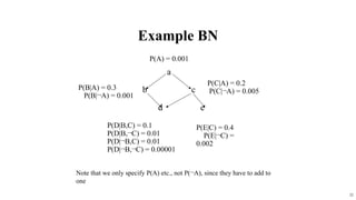
  • 32. 32 Example BN a b c d e P(C|A) = 0.2 P(C|?A) = 0.005 P(B|A) = 0.3 P(B|?A) = 0.001 P(A) = 0.001 P(D|B,C) = 0.1 P(D|B,?C) = 0.01 P(D|?B,C) = 0.01 P(D|?B,?C) = 0.00001 P(E|C) = 0.4 P(E|?C) = 0.002 Note that we only specify P(A) etc., not P(?A), since they have to add to one
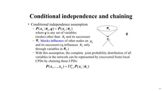
  • 33. 33 ? Conditional independence assumption C where q is any set of variables (nodes) other than and its successors C blocks influence of other nodes on and its successors (q influences only through variables in ) C With this assumption, the complete joint probability distribution of all variables in the network can be represented by (recovered from) local CPDs by chaining these CPDs: q Conditional independence and chaining
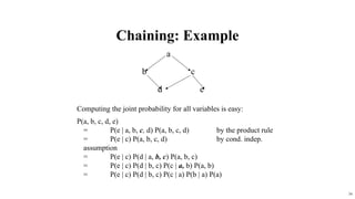
  • 34. 34 Chaining: Example Computing the joint probability for all variables is easy: P(a, b, c, d, e) = P(e | a, b, c, d) P(a, b, c, d) by the product rule = P(e | c) P(a, b, c, d) by cond. indep. assumption = P(e | c) P(d | a, b, c) P(a, b, c) = P(e | c) P(d | b, c) P(c | a, b) P(a, b) = P(e | c) P(d | b, c) P(c | a) P(b | a) P(a) a b c d e
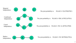
  • 35. 35 A B C Conditional Independence The joint probability is: P(A,B,C)= P(A)*P(B)*P(C) A B C The joint probability is: P(A,B,C)= P(B | A)*P(C|A)*P(A) C A B Causal Independence The joint probability is: P(A,B,C)= P(C |A, B)*P(A)*P(B) B A C Markov Independence The joint probability is: P(A,B,C)= P(C |B)*P(B|A)*P(A) Marginal Independence
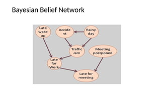
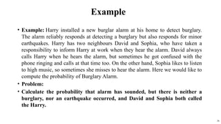
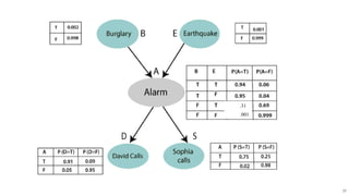
  • 36. Example ? Example: Harry installed a new burglar alarm at his home to detect burglary. The alarm reliably responds at detecting a burglary but also responds for minor earthquakes. Harry has two neighbours David and Sophia, who have taken a responsibility to inform Harry at work when they hear the alarm. David always calls Harry when he hears the alarm, but sometimes he got confused with the phone ringing and calls at that time too. On the other hand, Sophia likes to listen to high music, so sometimes she misses to hear the alarm. Here we would like to compute the probability of Burglary Alarm. ? Problem: ? Calculate the probability that alarm has sounded, but there is neither a burglary, nor an earthquake occurred, and David and Sophia both called the Harry. 36
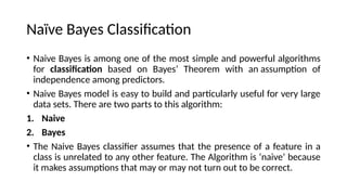
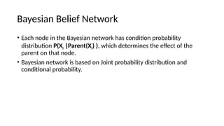
  • 38. ? We can write the events of problem statement in the form of probability: P[D, S, A, B, E], can rewrite the above probability statement using joint probability distribution: P[D, S, A, B, E]= P[D | S, A, B, E]. P[S, A, B, E] =P[D | S, A, B, E]. P[S | A, B, E]. P[A, B, E] = P [D| A]. P [ S| A, B, E]. P[ A, B, E] = P[D | A]. P[ S | A]. P[A| B, E]. P[B, E] = P[D | A ]. P[S | A]. P[A| B, E]. P[B]. P[E] Calculate the probability that alarm has sounded, but there is neither a burglary, nor an earthquake occurred, and David and Sophia both called the Harry. P(S, D, A, ?B, ?E) = P (S|A) *P (D|A)*P (A|?B, ?E) *P (?B) *P (?E). = 0.75* 0.91* 0.001* 0.998*0.999 = 0.00068045 38
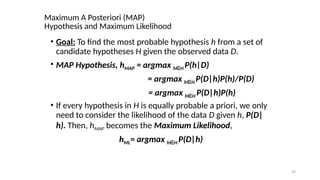
  • 39. 39 Maximum A Posteriori (MAP) Hypothesis and Maximum Likelihood ? Goal: To find the most probable hypothesis h from a set of candidate hypotheses H given the observed data D. ? MAP Hypothesis, hMAP = argmax h H ( P(h|D) = argmax h H ( P(D|h)P(h)/P(D) = argmax h H ( P(D|h)P(h) ? If every hypothesis in H is equally probable a priori, we only need to consider the likelihood of the data D given h, P(D| h). Then, hMAP becomes the Maximum Likelihood, hML= argmax h H ( P(D|h)