�ݺ�ߣ

Chapter 12
Inventory Management

Operations Management -- 5th Edition
Operations Management 5th Edition

Roberta Russell & Bernard W. Taylor, III

Beni Asllani
Copyright 2006 John Wiley & Sons, Inc. University of Tennessee at Chattanooga

Lecture Outline

 Elements of Inventory Management
 Inventory Control Systems
 Economic Order Quantity Models
 Quantity Discounts
 Reorder Point
 Order Quantity for a Periodic Inventory
System

Copyright 2006 John Wiley & Sons, Inc. 12-2

What Is Inventory?

 Stock of items kept to meet future
demand
 Purpose of inventory management
 how many units to order
 when to order


Types of Inventory

 Raw materials
 Purchased parts and supplies
 Work-in-process (partially completed)
products (WIP)
 Items being transported
 Tools and equipment


Inventory and Supply Chain
Management
 Bullwhip effect
 demand information is distorted as it moves away
from the end-use customer
 higher safety stock inventories to are stored to
compensate
 Seasonal or cyclical demand
 Inventory provides independence from vendors
 Take advantage of price discounts
 Inventory provides independence between
stages and avoids work stop-pages


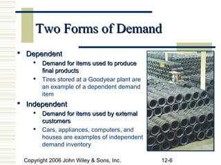
Two Forms of Demand
 Dependent
 Demand for items used to produce
final products
 Tires stored at a Goodyear plant are
an example of a dependent demand
item
 Independent
 Demand for items used by external
customers
 Cars, appliances, computers, and
houses are examples of independent
demand inventory


Inventory and Quality
Management

 Customers usually perceive quality
service as availability of goods they want
when they want them
 Inventory must be sufficient to provide
high-quality customer service in TQM


Inventory Costs

 Carrying cost
 cost of holding an item in inventory
 Ordering cost
 cost of replenishing inventory
 Shortage cost
 temporary or permanent loss of sales
when demand cannot be met


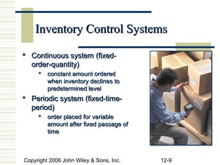
Inventory Control Systems

 Continuous system (fixed-
order-quantity)
 constant amount ordered
when inventory declines to
predetermined level
 Periodic system (fixed-time-
period)
 order placed for variable
amount after fixed passage of
time


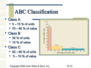
ABC Classification
 Class A
 5 – 15 % of units
 70 – 80 % of value
 Class B
 30 % of units
 15 % of value
 Class C
 50 – 60 % of units
 5 – 10 % of value


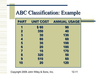
ABC Classification: Example
PART UNIT COST ANNUAL USAGE
1 $ 60 90
2 350 40
3 30 130
4 80 60
5 30 100
6 20 180
7 10 170
8 320 50
9 510 60
10 20 120


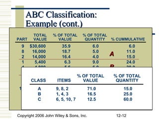
ABC Classification:
Example (cont.)
TOTAL % OF TOTAL % OF TOTAL
PART PART
VALUE UNIT COSTQUANTITY % CUMMULATIVE
VALUE ANNUAL USAGE
9 1
$30,600 $ 60
35.9 6.0 90 6.0
8 16,000
2 18.7
350 5.0 40 11.0
2 14,000 16.4 4.0
A 15.0
3 30 130
1 5,400 6.3 9.0 24.0
4 4
4,800 5.680 6.0 B60 30.0
3 5
3,900 4.630 10.0 100 40.0
% OF TOTAL % OF TOTAL
6 6
3,600
CLASS ITEMS
4.220 VALUE 18.0 180 58.0
QUANTITY
5 3,000
7 3.510 13.0 170 71.0
10 2,400
A 9, 8,2.8
2 12.0
71.0 C 83.0
8 320 50 15.0
7 1,700
B 1, 4,2.0
3 17.0
16.5 100.0
25.0
9
C 510
6, 5, 10, 7 12.5 60 60.0
$85,400
10 20 120
Example 10.1


Economic Order Quantity
(EOQ) Models

 EOQ
 optimal order quantity that will
minimize total inventory costs
 Basic EOQ model
 Production quantity model


Assumptions of Basic
EOQ Model

 Demand is known with certainty and
is constant over time
 No shortages are allowed
 Lead time for the receipt of orders is
constant
 Order quantity is received all at once


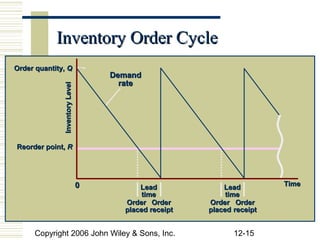
Inventory Order Cycle
Order quantity, Q
Demand
rate
Inventory Level

Reorder point, R

0 Lead Lead Time
time time
Order Order Order Order
placed receipt placed receipt


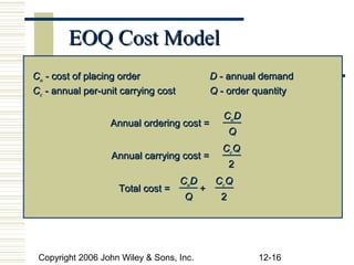
EOQ Cost Model
Co - cost of placing order D - annual demand
Cc - annual per-unit carrying cost Q - order quantity

Co D
Annual ordering cost =
Q
CcQ
Annual carrying cost =
2
CoD CcQ
Total cost = +
Q 2


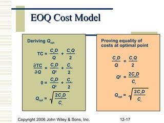
EOQ Cost Model

Deriving Qopt Proving equality of
costs at optimal point
Co D CcQ
TC = +
Q 2 Co D CcQ
=
∂TC CoD C Q 2
= + c
∂Q Q2 2 2CoD
Q = 2
C0 D Cc Cc
0= +
Q2 2
2CoD
2CoD Qopt =
Qopt = Cc
Cc


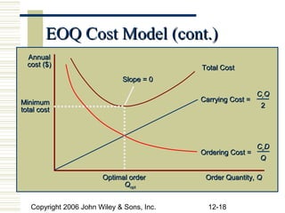
EOQ Cost Model (cont.)
Annual
cost ($) Total Cost
Slope = 0

CcQ
Minimum Carrying Cost =
2
total cost

CoD
Ordering Cost =
Q

Optimal order Order Quantity, Q
Qopt


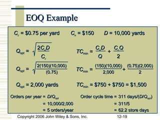
EOQ Example
Cc = $0.75 per yard Co = $150 D = 10,000 yards

2CoD CoD CcQ
Qopt = TCmin = +
Cc Q 2
2(150)(10,000) (150)(10,000) (0.75)(2,000)
Qopt = TCmin = +
(0.75) 2,000 2

Qopt = 2,000 yards TCmin = $750 + $750 = $1,500

Orders per year = D/Qopt Order cycle time = 311 days/(D/Qopt)
= 10,000/2,000 = 311/5
= 5 orders/year = 62.2 store days

Production Quantity
Model
 An inventory system in which an order is
received gradually, as inventory is
simultaneously being depleted
 AKA non-instantaneous receipt model
 assumption that Q is received all at once is relaxed
 p - daily rate at which an order is received over
time, a.k.a. production rate
 d - daily rate at which inventory is demanded


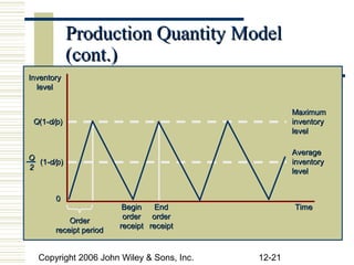
Production Quantity Model
(cont.)
Inventory
level

Maximum
Q(1-d/p) inventory
level

Average
Q
(1-d/p) inventory
2 level

0
Begin End Time
order order
Order
receipt receipt
receipt period


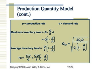
Production Quantity Model
(cont.)
p = production rate d = demand rate

Q
Maximum inventory level = Q - d
p
d
=Q1-
p 2CoD
Qopt = d
Q d Cc 1 - p
Average inventory level = 1-
2 p

CoD CcQ d
TC = + 1- p
Q 2


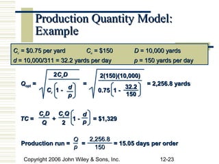
Production Quantity Model:
Example
Cc = $0.75 per yard Co = $150 D = 10,000 yards
d = 10,000/311 = 32.2 yards per day p = 150 yards per day

2CoD 2(150)(10,000)
Qopt = = = 2,256.8 yards
32.2
Cc 1 - d 0.75 1 -
p 150

Co D CcQ d
TC = + 1- p = $1,329
Q 2

Q 2,256.8
Production run = = = 15.05 days per order
p 150


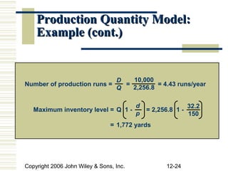
Production Quantity Model:
Example (cont.)

D 10,000
Number of production runs = = = 4.43 runs/year
Q 2,256.8

d 32.2
Maximum inventory level = Q 1 - = 2,256.8 1 -
p 150
= 1,772 yards


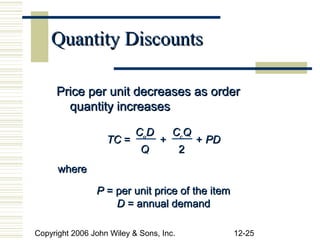
Quantity Discounts

Price per unit decreases as order
quantity increases

CoD CcQ
TC = + + PD
Q 2
where

P = per unit price of the item
D = annual demand


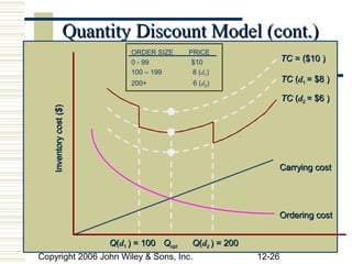
Quantity Discount Model (cont.)
ORDER SIZE PRICE
0 - 99 $10 TC = ($10 )
100 – 199 8 (d1)
200+ 6 (d2)
TC (d1 = $8 )

TC (d2 = $6 )
Inventory cost ($)

Carrying cost

Ordering cost

Q(d1 ) = 100 Qopt Q(d2 ) = 200

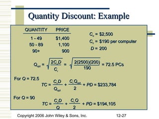
Quantity Discount: Example
QUANTITY PRICE
Co = $2,500
1 - 49 $1,400
Cc = $190 per computer
50 - 89 1,100
D = 200
90+ 900

2 Co D 2(2500)(200)
Qopt = = = 72.5 PCs
Cc 190

For Q = 72.5
CoD CcQopt
TC = + + PD = $233,784
Qopt 2

For Q = 90
Co D CcQ
TC = + + PD = $194,105
Q 2

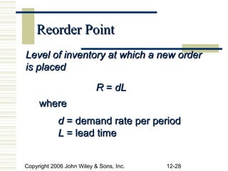
Reorder Point
Level of inventory at which a new order
is placed

R = dL
where
d = demand rate per period
L = lead time


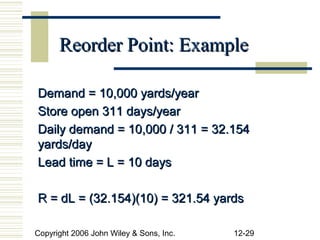
Reorder Point: Example

Demand = 10,000 yards/year
Store open 311 days/year
Daily demand = 10,000 / 311 = 32.154
yards/day
Lead time = L = 10 days

R = dL = (32.154)(10) = 321.54 yards


Safety Stocks
 Safety stock
 buffer added to on hand inventory during lead
time
 Stockout
 an inventory shortage
 Service level
 probability that the inventory available during
lead time will meet demand


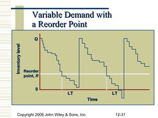
Variable Demand with
a Reorder Point
Q
Inventory level

Reorder
point, R

0
LT LT
Time


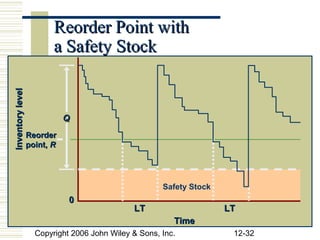
Reorder Point with
a Safety Stock
Inventory level

Q
Reorder
point, R

Safety Stock
0
LT LT
Time

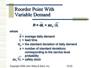
Reorder Point With
Variable Demand

R = dL + zσ d L
where
d = average daily demand
L = lead time
σd = the standard deviation of daily demand
z = number of standard deviations
corresponding to the service level
probability
zσd L = safety stock


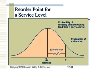
Reorder Point for
a Service Level
Probability of
meeting demand during
lead time = service level

Probability of
a stockout

Safety stock
zσ d L

dL R
Demand

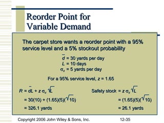
Reorder Point for
Variable Demand
The carpet store wants a reorder point with a 95%
service level and a 5% stockout probability
d = 30 yards per day
L = 10 days
σd = 5 yards per day

For a 95% service level, z = 1.65

R = dL + z σd L Safety stock = z σd L
= 30(10) + (1.65)(5)( 10) = (1.65)(5)( 10)
= 326.1 yards = 26.1 yards


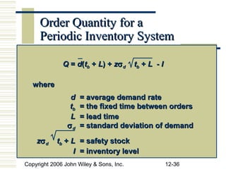
Order Quantity for a
Periodic Inventory System

Q = d(tb + L) + zσ d tb + L - I

where
d = average demand rate
tb = the fixed time between orders
L = lead time
σd = standard deviation of demand

zσ d tb + L = safety stock
I = inventory level

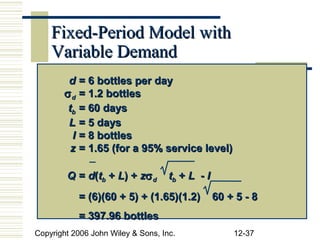
Fixed-Period Model with
Variable Demand
d = 6 bottles per day
σ d = 1.2 bottles
tb = 60 days
L = 5 days
I = 8 bottles
z = 1.65 (for a 95% service level)

Q = d(tb + L) + zσ d tb + L - I
= (6)(60 + 5) + (1.65)(1.2) 60 + 5 - 8
= 397.96 bottles

Copyright 2006 John Wiley & Sons, Inc.
All rights reserved. Reproduction or translation of this work beyond that
permitted in section 117 of the 1976 United States Copyright Act without
express permission of the copyright owner is unlawful. Request for further
information should be addressed to the Permission Department, John Wiley &
Sons, Inc. The purchaser may make back-up copies for his/her own use only and
not for distribution or resale. The Publisher assumes no responsibility for
errors, omissions, or damages caused by the use of these programs or from the
use of the information herein.


�ݺ�ߣ

Inventory management ch12

Recommended

More Related Content

What's hot (6)

Similar to Inventory management ch12 (20)

Inventory management ch12