Local SEO Keyword Strategies That Will Skyrocket Your Rankings In 2025.pdfKHM Anwar
╠²
What Are Harem Pants? Full Guide on Style, History & Modern FashionKerem BA┼×BU─×
╠²
Varun Hiremath ŌĆō Empowering Rural India Through Transformative Leadership & S...Varun Hiremath
╠²
Ad
Inventory management. humanities presentation ppt
1. Types of Inventory Situations
o Order repetitionŌĆöstatic versus dynamic situations.
o Demand distributionŌĆöcertainty, risk, and uncertainty.
o Stability of demand distributionŌĆöfixed or varying.
o Demand continuityŌĆösmoothly continuous or sporadic and
occurring as lumpy demand; independent.
o Lead-time distributionsŌĆöfixed or varying.
o Dependent or independent demand.
1
2. 2
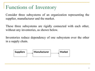
Functions of Inventory
Consider three subsystems of an organization representing the
supplier, manufacturer and the market.
These three subsystems are rigidly connected with each other,
without any inventories, as shown below.
Inventories reduce dependency of one subsystem over the other
in a supply chain.
Suppliers Manufacturer Market
3. Functions of Inventory (continued)
’üČ Production Planning ŌĆō level production.
’üČ Take advantage of quantity (price) discounts.
’üČ Protect against anticipated increase in prices.
’üČ Protect against anticipated shortages.
3
4. Inventory Related Costs
o Costs of ordering
o Costs of setups and changeovers
o Costs of carrying inventory
o Costs of discounts
o Out-of-stock costs
o Costs of running the inventory system
4
5. 5
Data for Inventory Problems
ŌĆó D: Annual Demand (units per year)
ŌĆó C: Unit Price (purchase price of the item)
ŌĆó S: Ordering or Setup Cost per Order
ŌĆó H: Inventory Holding (Carrying) Cost/unit per year
ŌĆó i: H may be given as i percent of C
ŌĆó TC: Total Annual Cost
ŌĆó TVC: Total Annual Variable Cost
ŌĆó Q: Order Quantity
ŌĆó EOQ: Economic Order Quantity (optimal value of Q)
7. 7
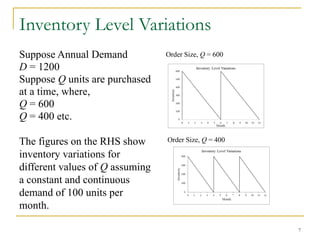
Inventory Level Variations
Suppose Annual Demand
D = 1200
Suppose Q units are purchased
at a time, where,
Q = 600
Q = 400 etc.
The figures on the RHS show
inventory variations for
different values of Q assuming
a constant and continuous
demand of 100 units per
month.
Order Size, Q = 600
Order Size, Q = 400
8. 8
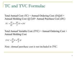
TC and TVC Formulae
Total Annual Cost (TC) = Annual Ordering Cost (D/Q)S +
Annual Holding Cost (Q/2)H+ Annual Purchase Cost (DC)
Total Annual Variable Cost (TVC) = Annual Ordering Cost +
Annual Holding Cost
Note: Annual purchase cost is not included in TVC.
H
Q
S
Q
D
TVC
2
’Ć½
’ĆĮ
DC
H
Q
S
Q
D
TC ’Ć½
’Ć½
’ĆĮ
2
9. 9
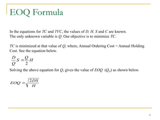
EOQ Formula
In the equations for TC and TVC, the values of D, H, S and C are known.
The only unknown variable is Q. Our objective is to minimize TC.
TC is minimized at that value of Q, where, Annual Ordering Cost = Annual Holding
Cost. See the equation below.
Solving the above equation for Q, gives the value of EOQ (QO) as shown below.
H
Q
S
Q
D
2
’ĆĮ
H
DS
EOQ
2
’ĆĮ
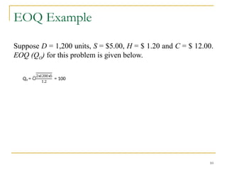
10. EOQ Example
Suppose D = 1,200 units, S = $5.00, H = $ 1.20 and C = $ 12.00.
EOQ (QO) for this problem is given below.
10
Qo = ÓȦ
2ŌłŚ
1200ŌłŚ
5
1.2
= 100
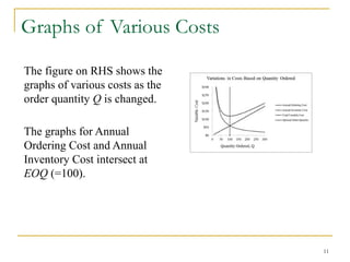
11. Graphs of Various Costs
The figure on RHS shows the
graphs of various costs as the
order quantity Q is changed.
The graphs for Annual
Ordering Cost and Annual
Inventory Cost intersect at
EOQ (=100).
11
12. 12
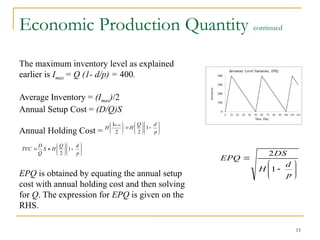
Economic Production Quantity
The economic production quantity (EPQ) model is used in
manufacturing situations where inventory is replenished at a
finite rate given by the production rate of the item under
consideration.
We define two more variables:
p: Production rate per day (daily production)
d: Demand rate per day (daily demand)
Note: p and d must be defined in the same time unit. For example
these could be weekly instead of daily rates.
13. 13
Economic Production Quantity continued
Suppose
p = 50 units/day
d = 10 units/day
EPQ = 500 (production quantity, Q); Note: the optimal value of
Q is EPQ or QP
In this case we will need 10 days to produce 500 units
(EPQ/p = 500/50).
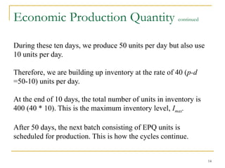
14. Economic Production Quantity continued
During these ten days, we produce 50 units per day but also use
10 units per day.
Therefore, we are building up inventory at the rate of 40 (p-d
=50-10) units per day.
At the end of 10 days, the total number of units in inventory is
400 (40 * 10). This is the maximum inventory level, Imax.
After 50 days, the next batch consisting of EPQ units is
scheduled for production. This is how the cycles continue.
14
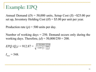
16. Example: EPQ
Annual Demand (D) = 50,000 units, Setup Cost (S) =$25.00 per
set up, Inventory Holding Cost (H) = $5.00 per unit per year.
Production rate (p) = 500 units per day.
Number of working days = 250. Demand occurs only during the
working days. Therefore, (d) = 50,000/250 = 200.
EPQ (QP) = 912.87 =
Imax = 548.
16
17. 17
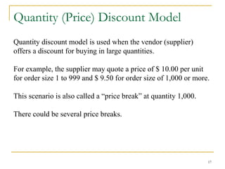
Quantity (Price) Discount Model
Quantity discount model is used when the vendor (supplier)
offers a discount for buying in large quantities.
For example, the supplier may quote a price of $ 10.00 per unit
for order size 1 to 999 and $ 9.50 for order size of 1,000 or more.
This scenario is also called a ŌĆ£price breakŌĆØ at quantity 1,000.
There could be several price breaks.
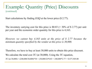
18. Example: Quantity (Price) Discounts
(continued)
Start calculations by finding EOQ at the lower price ($ 2.77).
The inventory carrying cost for this price is $0.83 (= 30% of $ 2.77) per unit
per year and the economic order quantity for this price is 4,163.
However, we cannot buy 4,163 units at the price of $ 2.77 because the
minimum quantity specified by the vendor at this price is 30,000.
Therefore, we have to buy at least 30,000 units to obtain this price discount.
We calculate the total cost TC (at 30,000). Using the TC equation,
TC (at 30,000) = (240,000/30,000)*30 + (30,000/2)*0.83 + 240,000*2.77 = $ 677,505.00
18
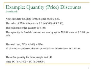
19. Example: Quantity (Price) Discounts
(continued)
Now calculate the EOQ for the higher price $ 2.80.
The value of H for this price is $ 0.84 (30% of $ 2.80).
The economic order quantity is 4,140.
This quantity is feasible because we can by up to 29,999 units at $ 2.80 per
unit.
The total cost, TC(at 4,140) will be:
TC (at 4,140) = = (240,000/4,140)*30 + (4,140/2)*0.84 + 240,000*2.80 = $ 675,477.93.
The order quantity for this example is 4,140
since TC (at 4,140) < TC (at 30,000).
19
20. ABC Analysis
Some materials are more important than others.
Importance can be established in the following two
ways:
o Material Criticality
o Annual Dollar Volume of Materials
20
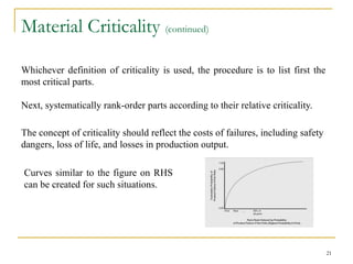
21. Material Criticality (continued)
Whichever definition of criticality is used, the procedure is to list first the
most critical parts.
Next, systematically rank-order parts according to their relative criticality.
The concept of criticality should reflect the costs of failures, including safety
dangers, loss of life, and losses in production output.
Curves similar to the figure on RHS
can be created for such situations.
21
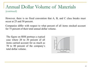
22. Annual Dollar Volume of Materials
(continued)
However, there is no fixed convention that A, B, and C class breaks must
occur at 25 and 50 percent.
Companies differ with respect to what percent of all items stocked account
for 75 percent of their total annual dollar volume.
The figure on RHS portrays a typical
case where 20 to 30 percent of all
items carried account for as much as
70 to 80 percent of the companyŌĆÖs
total dollar volume.
22
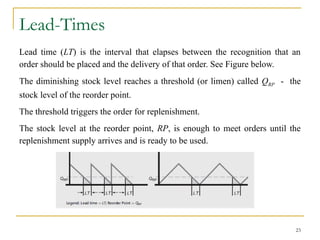
23. Lead-Times
Lead time (LT) is the interval that elapses between the recognition that an
order should be placed and the delivery of that order. See Figure below.
The diminishing stock level reaches a threshold (or limen) called QRP - the
stock level of the reorder point.
The threshold triggers the order for replenishment.
The stock level at the reorder point, RP, is enough to meet orders until the
replenishment supply arrives and is ready to be used.
23
24. Lead-Times (continued)
Eight lead-time (LT) considerations that apply to EOQ or EPQ or
both:
’āś The amount of time required to recognize the need to reorder.
’āś The interval for doing whatever clerical work is needed to
prepare the order.
’āś Mail, e-mail, EDI, or telephone intervals to communicate with
the supplier (or suppliers) and to place the order(s).
’āś Time that takes the supplierŌĆÖs organization to react to the
placement of an order?
24
25. Lead-Times (continued)
’āś Delivery time including loading, transit, and unloading.
’āś Processing of delivered items by the receiving department.
’āś Inspection to be sure items match specifications.
’āś Time delays in updating records The effect of such delays on
the production schedule must be considered.
The eight lead-time components are added to get the lead time.
Lead times are usually variable.
Safety stocks may be increased to deal with variable lead times.
25
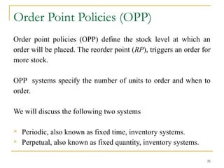
26. Order Point Policies (OPP)
Order point policies (OPP) define the stock level at which an
order will be placed. The reorder point (RP), triggers an order for
more stock.
OPP systems specify the number of units to order and when to
order.
We will discuss the following two systems
’āś Periodic, also known as fixed time, inventory systems.
’āś Perpetual, also known as fixed quantity, inventory systems.
26
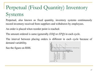
27. Perpetual (Fixed Quantity) Inventory
Systems
Perpetual, also known as fixed quantity, inventory systems continuously
record inventory received from suppliers and withdrawn by employees.
An order is placed when reorder point is reached.
The amount ordered is same (generally EOQ or EPQ) in each cycle.
The interval between placing orders is different in each cycle because of
demand variability.
See the figure on RHS.
27
28. Reorder Point and Safety (Buffer) Stock
Shortages occur whenever actual demand in the lead-time period exceeds QRP.
The likelihood of a shortage will be decreased by increasing the value of
safety( buffer) stock.
Determining safety (buffer) stock level requires an economic balancing
situation between the cost of going out of stock versus the cost of carrying
more inventory.
The large buffer stock means that the carrying cost of stock is high to make
sure that the actual cost of stock-outages is small.
The stock level of the reorder point (QRP) is equal to the expected (average)
demand during the lead time period plus the safety stock (SS) quantity.
Thus,
28
QRP = LT + SS
29. Expected Demand During Lead Time
The expected demand during lead time is a function of average demand per
day (d) and the magnitude of lead time (LT) and is determined as
It may be noted that calculation of demand during lead time becomes
complex if lead time also varies.
29
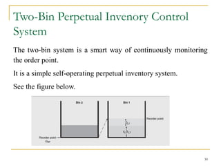
30. Two-Bin Perpetual Invenory Control
System
The two-bin system is a smart way of continuously monitoring
the order point.
It is a simple self-operating perpetual inventory system.
See the figure below.
30