�ݺ�ߣ

Sorting
Dr. Shaukat Wasi and Dr. Imran Jami
Material taken from Brooks/Cole and
GeeksforGeeks

Sorting
• In computer science, a sorting algorithm is an algorithm that puts elements of a list into
an order.
• The most frequently used orders are numerical order and lexicographical order, and either
ascending or descending.
• Formally, the output of any sorting algorithm must satisfy two conditions:
• The output is in monotonic order (each element is no smaller/larger than the previous
element, according to the required order).
• The output is a permutation (a reordering, yet retaining all of the original elements) of the
input.
[Wikipedia]

Sorting Concepts
• Sorting algorithms are classified as internal or external
• Internal sort holds all data in primary memory during the sorting process
• External sort uses primary memory for data currently sorted, and secondary storage
for data that did not fit in primary storage
• Knuth identified five classifications: insertion, selection, exchanging, merging, and
distribution
[Brooks/Cole
Thompson Learning]

Sorting Concepts
• Sort efficiency measures relative efficiency of the sort, estimating the number of comparisons
and moves required to order an unordered list
• A Sort Pass traverses data through a portion or the entire list
• Sort order may be ascending or descending
• Sort stability indicates whether data with equal keys maintain relative input order in the output
[Brooks/Cole
Thompson Learning]

Figure 11-2 – Sort Stability
[Brooks/Cole
Thompson Learning]

Sorting Concepts
• Sorting algorithms are classified as internal or external
• Internal sort holds all data in primary memory during the sorting process
• External sort uses primary memory for data currently sorted, and secondary storage
for data that did not fit in primary storage
• Knuth identified five classifications: insertion, selection, exchanging, merging, and
distribution

Selection Sort
Select smallest element from unsorted list and exchange with element at beginning
of unsorted list
Efficiency: O(n2)
Best/Worst/Average Case Complexity is Same
Not Stable
Simple and Easy

Algorithm
11-3
Selection
Sort
• algorithm selectionSort (ref list <array>, val last <index>)
• current = 0
• loop (current < last)
• smallest = current
• walker = current + 1
• loop (walker <= last)
• if (list[walker] < list[smallest])
• smallest = walker
• walker = walker + 1
• end loop
• Smallest selected: exchange with current element
• exchange (list, current, smallest)
• current = current + 1
• end loop
• return
• end selectionSort

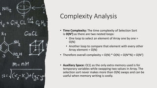
Complexity Analysis
• Time Complexity: The time complexity of Selection Sort
is O(N2) as there are two nested loops:
• One loop to select an element of Array one by one =
O(N)
• Another loop to compare that element with every other
Array element = O(N)
• Therefore overall complexity = O(N) * O(N) = O(N*N) = O(N2)
• Auxiliary Space: O(1) as the only extra memory used is for
temporary variables while swapping two values in Array. The
selection sort never makes more than O(N) swaps and can be
useful when memory writing is costly.

Stability??
• Selection sort swaps:
• Since 1 is minimum, swap 1 at position 4 with 7 at position 0.
• Swap 6 with 8
• Swap 9 at position 2 with 7 at position 3
• Swap 8 with 9
• In the first swap the ordering of the two ‘7s’ were changed. 7 at
position 0 was moved to position 4 that one position ahead from
another entry of 7 at position 3.
• Hence NOT Stable
0 1 2 3 4 5
7 8 9 7 1 6

Insertion Sort
– In each pass of an insertion sort, one or more pieces of data are inserted into the correct
location
– To sort an array of size N in ascending order
– iterate over the array and compare the current element (key) to its predecessor,
– if the key element is smaller than its predecessor, compare it to the elements before.
– Move the greater elements one position up to make space for the swapped element.
– Efficiency: O(n2)
– Best Case Complexity is O(n)
– Worst/Average Case Complexity is Same
– Stable
– Simple and Easy

Algorithm 11-1 Straight Insertion Sort
algorithm insertionSort (ref list <array>, val last <index>)
1. current = 1
2. loop (current <= last)
1. hold = list[current]
2. walker = current - 1
3. loop (walker >= 0 AND hold.key < list[walker].key)
1. list[walker + 1] = list[walker]
2. walker = walker - 1
4. end loop
5. list[walker + 1] = hold
6. current = current + 1
3. end loop
4. return
end insertionSort

Complexity Analysis
• Time Complexity: The time complexity of Insertion Sort is O(N2) as
there are two nested loops:
• Outer loop to traverse over the whole array for checking the
right placement of each element= O(N)
• Inner loop to compare that element with others to find it’s
right place= O(N)
• Therefore, overall complexity = O(N) * O(N) = O(N*N) = O(N2)
• Best Case Complexity is O(N) as the inner loop will not iterate in
any pass if all the items are already in sorted order.
temporary variables.

Stability??
Insertion Sort steps:
• 7, 8, and 9 are in right order so no change in first 3 iterations.
• 7 (at position 3) is matched with 9, then with 8, and then with 7 (at position 0)
and placed one position back before 8.
• 1 is matched in a similar order starting from 9 and placed at position 0.
• 6 is matched in reverse order and placed between 1 and 7 at position 1.
The two occurrences of 7 are placed in their original internal
ordering.
0 1 2 3 4 5
7 8 9 7 1 6

Bubble Sort
– Bubble Sort is the simplest sorting algorithm that works by repeatedly swapping the
adjacent elements if they are in the wrong order.
– traverse from left and compare adjacent elements and the higher one is placed at
right side.
– In this way, the largest element is moved to the rightmost end at first.
– This process is then continued to find the second largest and place it and so on until
the data is sorted.
– Efficiency: O(n2)
– Best Case Complexity is O(n)
– Worst/Average Case Complexity is Same
– Stable
– Simple and Easy

Algorithm 11-5 Bubble Sort
• algorithm bubbleSort (ref list <array>, val last <index>)
1.current = 0
2.sorted = false
3.loop (current <= last AND sorted false)
• Each iteration is one sort pass.
1.walker = last
2.sorted = true
3.loop (walker > current)
1.if (list[walker] < list[walker - 1])
• Any exchange means list is not sorted
1.sorted = false
2.exchange (list, walker, walker - 1)
2.end if
3.walker = walker - 1
4.end loop
5.current = current + 1
4.end loop
5.return
• end bubbleSort

Complexity Analysis
• Time Complexity: The time complexity of Bubble Sort is O(N2) as
there are two nested loops:
• One loop to push the largest element to the right = O(N)
• Another loop to track record of all elements to be checked
for their right position = O(N)
• Therefore, overall complexity = O(N) * O(N) = O(N*N) = O(N2)
• Best Case Complexity is O(N) as the outer loop will not iterate
more than once if no shuffling (bubbling) is done in the first pass
of the inner loop as it means the list is already sorted.
temporary variables.

Stability??
Bubble Sort steps:
• 9 moved to right (at position 5) in the first iteration. 7 (at position 3) moved to
position 2 and similarly 1 and 6 moves one position back.
• In the 2nd iteration, 8 moved to position 4. 7 (at position 2), 1 and 6 moved one
position back to positions 1, 2, and 3 respectively.
• 7 (at position 1) moved to position 3, and 1 and 6 moved one position back.
• 7 (at position 0) moved to position 2, and 1 and 6 moved one position back to reach
their right positions.
The two occurrences of 7 are placed in their original internal ordering.
0 1 2 3 4 5
7 8 9 7 1 6

Merge Sort
– Merge sort is defined as a sorting algorithm that works by dividing an
array into smaller subarrays, sorting each subarray, and then merging the
sorted subarrays back together to form the final sorted array.
– Efficiency: O(nlogn)
– Best/Worst/Average Case Complexity is Same
– Stable

Algorithm: Merge Sort
Algorithm mergeSort(S, C)
Input sequence S with n
elements, comparator C
Output sequence S sorted
according to C
if S.size() > 1
(S1, S2)  partition(S, n/2)
mergeSort(S1, C)
mergeSort(S2, C)
S  merge(S1, S2)
Algorithm merge(A, B)
Input sequences A and B with
n/2 elements each
Output sorted sequence of A  B
S  empty sequence
while A.isEmpty()  B.isEmpty()
if A.first().element() < B.first().element()
S.insertLast(A.remove(A.first()))
else
S.insertLast(B.remove(B.first()))
while A.isEmpty()
S.insertLast(A.remove(A.first()))
while B.isEmpty()
S.insertLast(B.remove(B.first()))
return S

Complexity Analysis
• Time Complexity: The time complexity of Merge Sort is O(NLogN):
• Since the list is divided into two parts repeatedly until single
elements lists are achieved so this repeated divide by 2
factor results in O(logN) complexity
• The n elements once divided into sub-lists are then merged
back to form a single sorted list. So merging of n elements
takes O(N) time and this merge is performed Log N times.
• Therefore, overall complexity = O(N) * O(LogN) = O(NLogN)
• Auxiliary Space: O(N) each element from the list is stored to some
auxiliary space during split.

Stability??
Merge Sort steps:
• Initially all elements are split one by one, and the order of their
positions remain same.
• While merging, the lists are merged in the same order as they were
split.
The two occurrences of 7 are placed in their original
internal ordering.
0 1 2 3 4 5
7 8 9 7 1 6

Quick Sort
– Quick sort is a sorting algorithm based on the Divide and Conquer algorithm that picks an element
as a pivot and partitions the given array around the picked pivot by placing the pivot in its correct
position in the sorted array.
– The key process in QuickSort is a partition().
– The target of partitions is to place the pivot (any element can be chosen to be a pivot) at its
correct position in the sorted array and
– put all smaller elements to the left of the pivot, and all greater elements to the right of the
pivot.
– Partition is done recursively on each side of the pivot after the pivot is placed in its correct
position and this finally sorts the array.
– Efficiency: O(nlogn)
– Best/Average Case Complexity is Same
– Worst Case Complexity is O(n2)
– Not Stable

Quick Sort
– Choice of Pivot:
– Always pick the first element as a pivot.
– Always pick the last element as a pivot
– Pick a random element as a pivot.
– Pick the middle as the pivot.
– Partition Algorithm
– The logic is simple, we start from the leftmost element and keep track of the index of smaller (or equal)
elements as i.
– While traversing, if we find a smaller element, we swap the current element with arr[i].
– Otherwise, we ignore the current element.
– As the partition process is done recursively, it keeps on putting the pivot in its actual position in the
sorted array.
– Repeatedly putting pivots in their actual position makes the array sorted.

Complexity Analysis
• Time Complexity: The time complexity of Quick Sort is O(NLogN):
• Since the list is divided into two parts repeatedly based on the
partition so this repeated divide by 2 factor results in O(logN)
complexity.
• However, after deciding the pivot the algorithm need to work on
both divided ends to further sort the items and hence the list is
processed from left to right finding pivots and setting them to right
position and this overall traversal over the list takes O(N) time.
• Therefore, overall complexity = O(N) * O(LogN) = O(NLogN)
• The choice of pivot may push the algorithm to worst case in which it
may perform similar to insertion sort.
• Auxiliary Space: O(1) in best case and O(N) in worst case.

Stability??
Quick Sort steps:
• The placement of pivot at it’s correct position after each pass of
sorting may result in changing the order of duplicates of an item
The positions of 7 are changed while placing 6 at it’s
correct position. Hence not stable.
0 1 2 3 4 5
7 8 9 7 1 6

�ݺ�ߣ

Lec 03 - Sorting.pptx

More Related Content

Lec 03 - Sorting.pptx