lec7.pdf
- 1. Biomedical Signal Processing Prof. Sudipta Mukhopadhyay Department of Electrical and Electronics Communication Engineering Indian Institute of Technology, Kharagpur Lecture - 07 Artifact Removal Now, we will learn about the removal of artifacts. (Refer ║▌║▌▀Ż Time: 00:19) So, to do that first let us have an overview of the system.
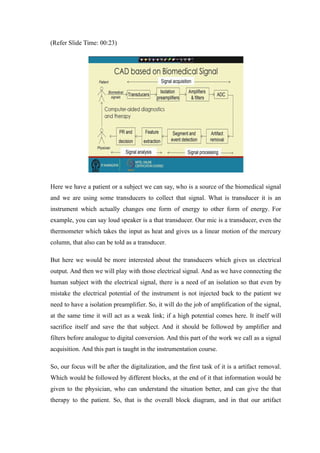
- 2. (Refer ║▌║▌▀Ż Time: 00:23) Here we have a patient or a subject we can say, who is a source of the biomedical signal and we are using some transducers to collect that signal. What is transducer it is an instrument which actually changes one form of energy to other form of energy. For example, you can say loud speaker is a that transducer. Our mic is a transducer, even the thermometer which takes the input as heat and gives us a linear motion of the mercury column, that also can be told as a transducer. But here we would be more interested about the transducers which gives us electrical output. And then we will play with those electrical signal. And as we have connecting the human subject with the electrical signal, there is a need of an isolation so that even by mistake the electrical potential of the instrument is not injected back to the patient we need to have a isolation preamplifier. So, it will do the job of amplification of the signal, at the same time it will act as a weak link; if a high potential comes here. It itself will sacrifice itself and save the that subject. And it should be followed by amplifier and filters before analogue to digital conversion. And this part of the work we call as a signal acquisition. And this part is taught in the instrumentation course. So, our focus will be after the digitalization, and the first task of it is a artifact removal. Which would be followed by different blocks, at the end of it that information would be given to the physician, who can understand the situation better, and can give the that therapy to the patient. So, that is the overall block diagram, and in that our artifact
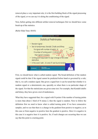
- 3. removal place a very important role, it is the first building block of the signal processing of the signal, or we can say it is doing the conditioning of the signal. Now, before getting into different artifact removal techniques first we should have some brush up of the statistics. (Refer ║▌║▌▀Ż Time: 04:03) First, we should know what is called random signal. The broad definition of the random signal could be that if the signal cannot be predicted before hand or governed by a rule; that is, we call a random signal. But given a signal how it can be tested that whether it is random signal or a deterministic one, specially so when there is no particular shape of the signal. For that the statisticians are given some test. For example, that Kendall challis and kitney, they have given a test of randomness. What they have suggested that, for a signal with N points if the number of turning points is more than about 2 third of N minus 2, then the signal is random. Now to follow the definition first we need to know what is called turning point. If we have consecutive samples, and we see that there is a change in the gradient from positive to negative, as in this case or from negative to positive here the gradient is positive. Here it is negative in this case it is negative here it is positive. So, if such changes are occurring then we can say that this point is a turning point.
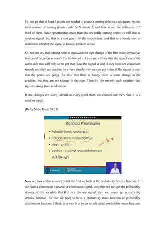
- 4. So, we get that at least 3 points are needed to create a turning point in a sequence. So, the total number of turning points could be N minus 2, and here as per the definition if 2 third of them, those opportunities more than that are really turning points we call that as random signal. So, that is a test given by the statisticians, and that is a handy tool to determine whether the signal at hand is random or not. So, we can say that turning point is equivalent to sign change of the first order derivative, that could be given as another definition of it. Later we will see that the waveform of the word safe that will help us to get that, how the signal is and if they both are consonant sounds and they are random. In a very simple way we can get it that if the signal is mod that the points are going like this, that there is hardly there is some change in the gradient, but they are not change in the sign. Then for the smooth such variation that signal is away from randomness. If the changes are sharp, almost at every point then, the chances are there that it is a random signal. (Refer ║▌║▌▀Ż Time: 08:31) Now we look at that in more detail the first we look at the probability density function. If we have a continuous variable or continuous signal, then that we can get the probability density of that variable. But if it is a discrete signal, then we cannot get actually the density function, for that we need to have a probability mass function or probability distribution function. I think in a way it is better to talk about probability mass function.
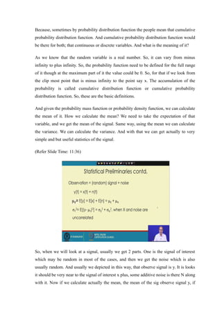
- 5. Because, sometimes by probability distribution function the people mean that cumulative probability distribution function. And cumulative probability distribution function would be there for both; that continuous or discrete variables. And what is the meaning of it? As we know that the random variable is a real number. So, it can vary from minus infinity to plus infinity. So, the probability function need to be defined for the full range of it though at the maximum part of it the value could be 0. So, for that if we look from the clip most point that is minus infinity to the point say x. The accumulation of the probability is called cumulative distribution function or cumulative probability distribution function. So, these are the basic definitions. And given the probability mass function or probability density function, we can calculate the mean of it. How we calculate the mean? We need to take the expectation of that variable, and we get the mean of the signal. Same way, using the mean we can calculate the variance. We can calculate the variance. And with that we can get actually to very simple and but useful statistics of the signal. (Refer ║▌║▌▀Ż Time: 11:36) So, when we will look at a signal, usually we get 2 parts. One is the signal of interest which may be random in most of the cases, and then we get the noise which is also usually random. And usually we depicted in this way, that observe signal is y. It is looks it should be very near to the signal of interest x plus, some additive noise is there N along with it. Now if we calculate actually the mean, the mean of the sig observe signal y, if
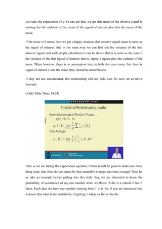
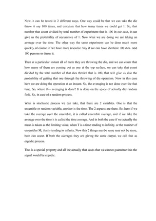
- 6. you take the expectation of y we can get that, we get that mean of the observe signal is nothing but the addition of the mean of the signal of interest plus that the mean of the noise. If the noise is 0 mean, then we get a happy situation that observe signal mean is same as the signal of interest. And in the same way we can find out the variance of the that observe signal, and with simple calculation it can be shown that it is same as the sum of the variance of the that signal of interest; that is, sigma x square plus the variance of the noise. When however, there is an assumption here in both this case cases, that there is signal of interest x and the noise, they should be uncorrelated. If they are not uncorrelated, this relationship will not hold true. So now, let us move forward. (Refer ║▌║▌▀Ż Time: 14:24) Here ss we are taking the expectation operator, I think it will be good to make one more thing clear, that what do you mean by that ensemble average and time average? Now let us take an example before getting into this slide. Say, we are interested to know the probability of occurrence of say one number when we throw. A die is a cuboid it has 6 faces. Each face we have one number varying from 1 to 6. So, if you are interested that to know that what is the probability of getting 1 when we throw the die.
- 7. Now, it can be tested in 2 different ways. One way could be that we can take the die throw it say 100 times, and calculate that how many times we could get 1. So, that number that count divided by total number of experiment that is 100 in our case, it can give us the probability of occurrence of 1. Now what we are doing we are taking an average over the time. The other way the same experiment can be done much more quickly of course, if we have more resource. Say if we can have identical 100 dies. And 100 persons to throw it. Then at a particular instant all of them they are throwing the die, and we can count that how many of them are coming out as one at the top surface, we can take that count divided by the total number of that dies thrown that is 100, that will give us also the probability of getting that one through the throwing of die operation. Now in this case here we are doing the operation at an instant. So, the averaging is not done over the that time. So, where this averaging is done? It is done on the space of actually did random field. So, in case of a random process. What is stochastic process we can take, that there are 2 variables. One is that the ensemble or random variable, another is the time. The 2 aspects are there. So, here if we take the average over the ensemble, it is called ensemble average, and if we take the average over the time it is called the time average. And in both the case if we actually the mean is taken as the limiting value, when T is a time tending to infinity, or the number of ensembles M; that is tending to infinity. Now this 2 things maybe same may not be same, both can occur. If both the averages they are giving the same output, we call that as ergodic process. That is a special property and all the actually that cases that we cannot guarantee that the signal would be ergodic.
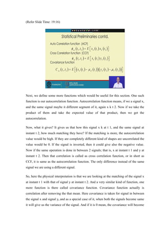
- 8. (Refer ║▌║▌▀Ż Time: 19:16) Next, we define some more functions which would be useful for this section. One such function is our autocorrelation function. Autocorrelation function means, if we a signal x, and the same signal maybe it different segment of it, again x k t 2. Now if we take the product of them and take the expected value of that product, then we get the autocorrelation. Now, what it gives? It gives us that how this signal x k at t 1, and the same signal at instant t 2, how much matching they have? If the matching is more, the autocorrelation value would be high. If they are completely different kind of shapes are uncorrelated the value would be 0. If the signal is inverted, then it could give also the negative value. Now if the same operation is done in between 2 signals; that is, x at instant t 1 and y at instant t 2. Then that correlation is called as cross correlation function, or in short as CCF, it is same as the autocorrelation function. The only difference instead of the same signal we are using a different signal. So, here the physical interpretation is that we are looking at the matching of the signal x at instant t 1 with that of signal y at instant t 2. And a very similar kind of function, one more function is there called covariance function. Covariance function actually is correlation after removing the that mean. Here covariance is taken for signal in between the signal x and signal y, and as a special case of it, when both the signals become same it will give us the variance of the signal. And if it is 0 mean, the covariance will become
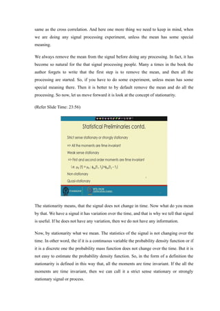
- 9. same as the cross correlation. And here one more thing we need to keep in mind, when we are doing any signal processing experiment, unless the mean has some special meaning. We always remove the mean from the signal before doing any processing. In fact, it has become so natural for the that signal processing people. Many a times in the book the author forgets to write that the first step is to remove the mean, and then all the processing are started. So, if you have to do some experiment, unless mean has some special meaning there. Then it is better to by default remove the mean and do all the processing. So now, let us move forward it is look at the concept of stationarity. (Refer ║▌║▌▀Ż Time: 23:56) The stationarity means, that the signal does not change in time. Now what do you mean by that. We have a signal it has variation over the time, and that is why we tell that signal is useful. If he does not have any variation, then we do not have any information. Now, by stationarity what we mean. The statistics of the signal is not changing over the time. In other word, the if it is a continuous variable the probability density function or if it is a discrete one the probability mass function does not change over the time. But it is not easy to estimate the probability density function. So, in the form of a definition the stationarity is defined in this way that, all the moments are time invariant. If the all the moments are time invariant, then we can call it a strict sense stationary or strongly stationary signal or process.
- 10. But getting all the moment same is same as that the probability distribution is remaining same over the time. Now as it is a very difficult proposition to calculate even all the moments, a simpler definition is given, and that is called weak sense stationary signal or weak sense stationary process. In this case instead of all the moments only the first 2 moments are taken that is a first order and the second order moments; that means, the mean of the signal and the variance of the signal. If they remain same, then we can tell the signal is weak sense stationary. And if any signal is not weak sense stationery; that means, the first 2 moments are varying over the time; that means, they cannot be strict sense stationary also. They are not strict sense stationary. So, such signals are called as non-stationary signal. So, the definition of non- stationary signal is a negative definition, you cannot have a direct definition of it. If anything is not stationary we call it as a non-stationary signal. However in nature if you look we will find all the signals are non-stationary. But it is more difficult to deal with the non-stationary signal. So, we need to somehow bring the assumption of stationarity. So, one more definition is created. If the signal does not change over a small period of time or small interval of time, we can call that signal as a quasi-stationary signal; that means, in case of a quasi-stationary signal within that interval that the mean and the variance are not changing much. So, that is the that gives us the definition of the quasi stationary signal, and we can take that segment of the sigma signal, and we can process it as a stationary signal.
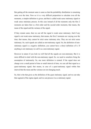
- 11. (Refer ║▌║▌▀Ż Time: 28:55) Here we can show some example of the stationary and non-stationary signal, if we look at the top graph, it is a stationary signal, if we look at in a small window, but if we look at the overall signal, we can get it very clearly that signal envelope is actually changing somewhere it is becoming close to 0, somewhere it is becoming very high. So, this signal as a as such is a non-stationary signal, but if we take a small window, we can say more or less the characteristic remains to be the same. So, we can also called it as a quasi-stationary signal. Now if we look at the same signal in a frequency domain, then also the same thing is depicted. For the top one here, that top plot here is a y axis is gives the magnitude of the signal, and x axis is giving the time. For the bottom graph; however, that x axis remains to be the time, and the y axis is giving the frequency. So, here you can say that we are using the short time fourier transform to get that the intervals what we have taken that we can take at any vertical line gives us the spectrum at that instant, and that remains to be very close or very similar within that one interval. So, that also convinces us about the assumptions what we have taken as quasi stationary. So, with that we complete the that preliminaries. And thank you. The next session we will start that how the artifacts are removed.