�ݺ�ߣ

Material Balance for Oil Reservoirs
Md. Mehedi Hasan
Lecturer, Dept. of PME
Jessore University of Science and Technology (JUST)

Uses of material balance
Material balance calculations can be used to:
 Determine original oil and gas in place in the reservoir;
 Determine original water in place in the aquifer;
 Estimate expected oil and gas recoveries as a function of pressure
decline in a closed reservoir producing by depletion drive, or as a
function of water influx in a water-drive reservoir;
 Predict future behavior of a reservoir (production rates, pressure
decline, and water influx);
 Verify volumetric estimates of original fluids in place;
 Verify future production rates and recoveries predicted by
decline-curve analysis;
 Determine which primary producing drive mechanisms are
responsible for a reservoir's observed behavior, and quantify the
relative importance of each mechanism;
 Evaluate the effectiveness of a water drive;
 Study the interference of fields sharing a common aquifer.

Assumption for Material Balance
 The material balance equations considered assume tank type
behavior at any given datum depth
 The reservoir is considered to have the same pressure and fluid
properties at any location in the reservoir.
 This assumption is quite reasonable provided that quality
production and static pressure measurements are obtained.
 Reservoir consider homogeneous porosity permeability

The Material Balance Equation
The equation can be written on volumetric basis
as:
Initial volume = volume remaining + volume removed
Before deriving the material balance, it is convenient
to denote certain terms by symbols for brevity. The
symbols used conform where possible to the standard
nomenclature adopted by the Society of
Petroleum Engineers (SPE)

Basic Principle
p1 > p2 p3 p4
> >
Undersaturated
oil
Bubble
point
Expanding
Gas Cap
Liquid shrinking
due to liberation
of dissolved gas
Oil
+
dissolved
gas
Initial gas cap Expanded gas cap
Expanded of oil +
dissolved gas
Reduction in PV due to
increased grain packing
and connate water
expansion
Pinit P
>

Terms Symbols
Initial reservoir pressure, psi Pi
Change in reservoir pressure = pi − p, psi Δp
Bubble point pressure, psi Pb
Initial (original) oil in place, STB N
Cumulative oil produced, STB Np
Cumulative water produced, bbl Wp
Cumulative gas produced, scf Gp
Cumulative gas-oil ratio, scf/STB Rp
Instantaneous gas-oil ratio, scf/STB GOR
Initial gas solubility, scf/STB Rsi
Gas solubility, scf/STB Rs

Terms Symbols
Initial oil formation volume factor, bbl/STB Boi
Oil formation volume factor, bbl/STB Bo
Initial gas formation volume factor, bbl/scf Bgi
Gas formation volume factor, bbl/scf Bg
Cumulative water injected, STB Winj
Cumulative gas injected, scf Ginj
Cumulative water influx, bbl We
Ratio of initial gas-cap-gas reservoir volume to
initial reservoir oil volume , bbl/bbl
m
Initial gas-cap gas, scf G
Pore volume, bbl P.V

Terms Symbols
Water compressibility, psi−1 cw
Formation (rock) compressibility, psi−1 cf
Gas formation volume factor of the gas cap gas ,bbl/scf Bg c
Gas formation volume factor of the solution gas
,bbl/scf
Bg s
Cumulative gas production from gas cap Gpc
Cumulative gas production from solution gas
. Gps

In this lecture we will derive the material balance as a
volumetric balance. Material balance is also a critical step
in modern reservoir simulation where a mass balance of
components within the different fluid phases is generally
performed.
Pinit P
>
A
B
Oil +
dissolved
gas
Gas cap
C
wl = Expansion of oil + originally
dissolved gas (B) (rb)
+ Expansion of gascap gas(A)(rb)
+ Reduction in PV due to
expansion of connate water
and tighter grain packing(C)(rb)
that the volume balance is written in terms of fluid at
oir conditions or as underground withdrawl and
pansion.

Data available to do material balance
Production Data
Np = Cumulative oil volume produced (stb)
Rp = Cumulative gas-oil ratio
=
PVT properties
Bo = Oil FVF (bbl/STB)
Bg = Gas FVF (cu.ft/SCF)
Bw = Water FVF(bbl/STB)
Cw = Compressibility of water (psi-1
)
Rso = Solution Gas-Oil Ratio
Reservoir properties
Cf = Rock Compressibility
Swi = Connate water saturation
(stb)
produced
oil
of
volume
Cum.
(scf)
produced
gas
of
volume
Cum.

Data available to do material balance (Cont.)
N = Initial volume of oil in reservoir (rb)
= (stb)
m = Initial gas cap
=
These are listed as other parameters because these may
either be known by wireline logs, reservoir modeling etc.
Or they may be the objective of the material balance
computation.
(rb)
oil
of
n volume
hydrocarbo
Initial
(rb)
gap
gas
of
n volume
hydrocarbo
Initial
oi
wc B
S
V /
)
1
( 




Derivation of the material balance
Expansion of the oil + liberated gas
mponents:
nsion of oil:
Initial Oil = N (stb)
Initial oil at reservoir conditions = N Boi (rb)
Volume of oil at reduced pressure p = N Bo (rb)
Net oil expansion = N(Bo-Boi) (rb)
nsion of liberated gas:
issolved at initial condition = NRsi (scf)
issolved at reduced pressure p = NRs (scf)
ated gas = N(Rsi-Rs) (scf)
me of gas at reservoir conditions= N(Rsi-Rs)Bg (rb)

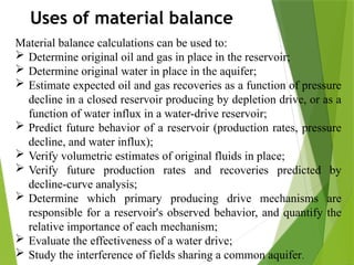
Derivation of the material balance
Expansion of the gas cap gas
Expansion of the gascap gas = gascap gas (at p) –gascap (at pi)
RB
SCF
RB
SCF
B
B
mNB
p
at
gas
of
Amount
SCF
SCF
RB
RB
B
mNB
G
or
RB
SCF
RB
STB
SCF
SCF
mNB
gas
gascap
of
volume
total
The
g
gi
oi
gi
oi
oi
]
[
]
[
1
)
(
]
[
1
]
[
1
]
[
]
[









)
3
.
3
(
)
(
)
1
(
]
[





RB
B
B
mNB
RB
mNB
B
B
mNB
gas
gascap
the
of
Expansion
gi
g
oi
oi
gi
g
oi






Derivation of the material balance (Cont.)
Change in the HCPV due to the connate water
expansion & pore volume reduction
p
S
c
S
c
NB
m
p
c
S
c
S
mNBoi
NBoi
p
c
S
c
S
HCPV
p
c
S
c
V
p
V
c
S
V
c
S
V
vol
water
connate
the
V
p
V
c
V
c
S
HCPV
vol
pore
total
the
V
dV
dV
HCPV
d
wc
f
wc
w
oi
f
wc
w
w
f
wc
w
w
f
wc
w
f
f
f
wc
f
w
wc
f
w
f
f
w
w
w
f
f
w







































)
1
(
)
1
(
)
(
)
1
(
)
(
)
1
(
)
(
)
(
.
)
(
)
1
/(
.
)
(

Underground withdrawal
]
)
(
[
)
(
)
(
)
(
)
(
)
(
)
(
Pr
g
s
p
o
p
g
s
p
p
o
p
g
s
p
p
p
o
p
p
p
p
B
R
R
B
N
B
R
R
N
B
N
withdrawal
d
Undergroun
gas
RB
B
R
N
R
N
oil
RB
B
N
withdrawal
d
Undergroun
gas
SCF
R
N
oil
STB
N
surface
at
oduction













Withdrawal = Expansion of oil +originally (rb) dissolved gas (B)
(rb) + Expansion of gascap gas(A)(rb) + Reduction in HCPV due
to expansion of connate water and tighter grain packing(C)(rb)
�ݺ�ߣ: 15=12+13+14

The general expression for the material balance as
w
p
e
wc
f
wc
w
oi
gi
g
oi
g
s
si
oi
o
g
s
p
o
p
B
W
W
p
S
c
S
c
NB
m
B
B
mNB
B
R
R
N
B
B
N
B
R
R
B
N
)
(
)
1
(
)
1
(
)
1
(
)
(
)
(
]
)
(
[















)
7
.
3
(
)
(
1
)
1
(
1
)
(
)
(
]
)
(
[





w
p
e
wc
f
wc
w
gi
g
oi
g
s
si
oi
o
oi
g
s
p
o
p
B
W
W
p
S
c
S
c
m
B
B
m
B
B
R
R
B
B
NB
B
R
R
B
N








































p
measuring
difficulty
Main
p
V
c
dV
fluids
reservoir
of
Expansion
oduction
form
Simple
t
p
f
W
p
f
B
R
B
Note
e
g
s
o
:
Pr
:
)
,
(
)
(
,
,
:








Features of MBE
 It is zero dimensional, meaning that it is
evaluated at a point in the reservoir
 Lack of time dependence
 Pressure only appears explicitly in the water and
pore compressibility.
 Water influx is pressure and time depended
parameter
 The equation is always evaluated in the way it
was derived by comparing the current volumes at
pressure P to the original volumes at Pi. It is not
evaluated in steps –wise or differential fashion.

The general expression for the material balance as
w
p
e
wc
f
wc
w
oi
gi
g
oi
g
s
si
oi
o
g
s
p
o
p
B
W
W
p
S
c
S
c
NB
m
B
B
mNB
B
R
R
N
B
B
N
B
R
R
B
N
)
(
)
1
(
)
1
(
)
1
(
)
(
)
(
]
)
(
[















)
7
.
3
(
)
(
1
)
1
(
1
)
(
)
(
]
)
(
[





w
p
e
wc
f
wc
w
gi
g
oi
g
s
si
oi
o
oi
g
s
p
o
p
B
W
W
p
S
c
S
c
m
B
B
m
B
B
R
R
B
B
NB
B
R
R
B
N








































F
E Eg
E f w
w
p
e
w B
W
WeB 

where
)
12
.
3
(
)
( , 




w
e
w
f
g
o B
W
mE
mE
E
N
F 



STB
RB
p
S
c
S
c
B
m
E
STB
RB
B
B
B
E
STB
RB
B
R
R
B
B
E
RB
B
W
B
R
R
B
N
F
wc
f
wc
w
oi
w
f
gi
g
oi
g
g
s
si
oi
o
o
w
p
g
s
p
o
p


















)
1
(
)
1
(
]
[
)
1
(
]
[
)
(
)
(
]
[
]
)
(
[
,
Material Balance Expressed as a Liner Equation

 No initial gascap, negligible water influx
 With water influx eq(3.12) becomes
 Eq.(3.12) having a combination drive-all possible sources of energy.
0
& 
w
f c
c
)
13
.
3
(
)
12
.
3
.( 




o
NE
F
Eq 

)
14
.
3
(





o
e
o E
W
N
E
F


)
12
.
3
(
)
( , 




w
e
w
f
g
o B
W
mE
mE
E
N
F 



Material Balance Expressed as a Liner Equation (Cont.)

§ 3.4 Reservoir Drive Mechanisms
- Solution gas drive
- Gascap drive
-Natural water
drive
- Compaction drive
In terms of
-reducing the M.B to a compact form to
quantify reservoir performance
-determining the main producing
characteristics,
for example, GOR; water cut
-determining the pressure decline in the
reservoir
- estimating the primary recovery factor
Reservoir drive mechanism

Reservoir Drive Mechanisms
§ 3.5 Solution gas drive
(a) above the B.P. pressure (b) below the B.P.
pressure

Above the B.P. pressure
- no initial gascap, m=0
- no water flux, We=0 ; no water production, Wp=0
- Rs=Rsi=Rp
from eq.(3.7)
)
7
.
3
(
)
(
1
)
1
(
1
)
(
)
(
]
)
(
[





w
p
e
wc
f
wc
w
gi
g
oi
g
s
si
oi
o
oi
g
s
p
o
p
B
W
W
p
S
c
S
c
m
B
B
m
B
B
R
R
B
B
NB
B
R
R
B
N







































0
;
0
;
0
;
0
)
(
;
0
)
(
: 





 p
e
s
si
s
p W
W
m
R
R
R
R
Note
ility
compressib
weighted
saturation
effective
the
S
c
S
c
S
c
c
where
S
S
p
c
NB
B
N
or
p
B
B
B
p
B
B
B
p
S
c
S
c
S
c
NB
B
N
dp
dB
B
dp
dV
V
c
p
S
c
S
c
c
NB
B
N
p
S
c
s
c
B
B
B
NB
B
N
wc
f
w
w
o
o
e
wc
o
e
oi
o
p
oi
oi
o
oi
o
oi
wc
f
w
w
o
o
oi
o
p
o
o
o
o
o
wc
f
w
w
o
oi
o
p
wc
f
wc
w
oi
oi
o
oi
o
p








































,
1
1
)
18
.
3
(
)
(
)
(
)
17
.
3
(
)
1
(
1
1
)]
1
(
[
]
1
)
(
)
(
[











Exercise3.1 Solution gas drive, undersaturated oil reservoir
Determine R.F.
Solution:
FromTable2.4(p.65)
2
.
0
10
6
.
8
10
3
)
65
.
(
4
.
2
1
6
1
6












w
f
w
b
i
S
psi
c
psi
c
p
table
PVT
p
p
p
if
STB
RB
B
psi
p
STB
RB
B
psi
p
ob
b
oi
i
12511
,
3330
2417
.
1
,
4000




1
6
10
3
.
11
)
3330
4000
(
2417
.
1
2417
.
1
2511
.
1
1
1














psi
p
B
B
B
c
dp
dB
B
dp
dV
V
c
oi
oi
ob
o
o
o
o
o
o
Eq(3.18)
%
5
.
1
015
.
0
)
3330
4000
(
10
8
.
22
2511
.
1
2417
.
1
.
.
6













p
c
B
B
N
N
F
R
p
c
NB
B
N
e
ob
oi
Pb
p
e
oi
o
p )
1
)(
1
/(
1
wc
f
w
w
o
o
S
c
S
c
S
c
Swc
Ce






Table 2.4 Field PVT
P(psia) Bo (Rb/STB) Rs(SCF/STB) Bg( Rb/SCF)
4000 (pi) 1.2417 510
3500 1.2480 510
3300 (pb) 1.2511 510 0.00087
3000 1.2222 450 0.00096
2700 1.2022 401 0.00107
2701 1.1822 352 0.00119
2702 1.1633 304 0.00137
1800 1.1450 257 0.00161
2703 1.1287 214 0.00196
1200 1.1115 167 0.00249
2704 1.0940 122 0.00339
2705 1.0763 78 0.00519
300 1.0583 35 0.01066

%
7
.
16
167
.
0
4000
3330
4000
%
Pr
10
8
.
22
)
10
6
.
8
2
.
0
10
3
8
.
0
10
3
.
11
(
2
.
0
1
1
1
:
6
6
6
6

























p
drop
essure
S
c
S
c
S
c
c
Note
wc
f
w
w
o
o
e
Ce= Saturation weighted compressibility

Bg and E as Function of Pressure
E= Gas expansion

Producing Gas-oil Ratio (R) as Function of Pressure

Below B.P. pressure (Saturation oil)
P<Pb =>gas liberated from saturated oil
1
6
1
6
1
6
1
6
1
6
10
6
.
8
10
3
10
3
.
11
10
300
10
300
3300
1
1
1























psi
c
psi
c
psi
c
psi
c
psi
P
p
c
f
w
o
g
b
g

Exercise 3.2 Solution gas drive; below bubble point pressure
Reservoir-described in exercise 3.1
Pabandon = 900psia
(1) R.F = f(Rp)? Conclusion?
(2) Sg(free gas) = F(Pabandon)?
Solution:
(1) From eq(3.7)
)
7
.
3
(
)
(
1
)
1
(
1
)
(
)
(
]
)
(
[





w
p
e
wc
f
wc
w
gi
g
oi
g
s
si
oi
o
oi
g
s
p
o
p
B
W
W
p
S
c
S
c
m
B
B
m
B
B
R
R
B
B
NB
B
R
R
B
N







































developed
is
S
if
negligible
is
p
S
c
S
c
NB
W
W
cap
gas
initial
no
m
P
B
below
gas
solution
for
g
wc
f
wc
w
oi
p
e









)
1
(
0
;
0
0
.
.

Eq(3.7) becomes
)
20
.
3
(
]
)
(
)
[(
]
)
(
[ 




g
s
si
oi
o
g
s
p
o
p B
R
R
B
B
N
B
R
R
B
N 





201
344
00339
.
0
)
122
(
0940
.
1
00339
.
0
)
122
510
(
)
2417
.
1
0940
.
1
(
.
.
)
(
)
(
)
(
.
.
900
900




















p
p
p
p
p
g
s
p
o
g
s
si
oi
o
p
R
R
N
N
F
R
B
R
R
B
B
R
R
B
B
N
N
F
R
Conclusion:
Rp
RF
1

49
.
0
%
49
500
)
85
.
(
3
.
3
.
900




N
N
STB
SCF
R
p
Fig
From
p
p

mat_bal of reservoir engineering program.pptx

(2) the overall gas balance
)
21
.
3
(
)
1
(
)]
(
)
(
[
)
(
)
1
(
)
1
(
1





oi
wc
g
s
p
p
s
si
g
g
s
p
g
p
p
g
si
wc
g
oi
b
wc
wc
oi
NB
S
B
R
R
N
R
R
N
S
B
R
N
N
B
R
N
B
NR
S
S
NB
p
p
for
S
HCPV
volume
pore
S
NB

















liberated
gas in the
reservoir
total
amount
of gas
gas
produced
at surface
gas still
dissolved
in the oil
= − − -
4428
.
0
8
.
0
00339
.
0
2417
.
1
)]
122
500
(
49
.
0
)
122
510
[(
)
1
(
)]
(
)
[(
)
1
(
)]
(
)
(
[
















 wc
g
oi
s
p
p
s
si
oi
wc
g
s
p
s
si
g S
B
B
R
R
N
N
R
R
NB
S
B
R
R
Np
R
R
N
S

Water injection below bubble point Pressure

Exercise 3.3 (Cont.)
 To produced 10,000stb/d oil initial injection rate
4X10,000 = 40,000 rb/d water required
 70 % water needed to displace the liberated gas
 Above bubble point 1.2511x 10,000 =12500 b/d

Gascap Drive
 Under initial conditions the oil at the gas oil contract must be at
saturation or bubble point pressure.
 The oil further downdip becomes progressively less saturated at the
higher pressure and temperature.
 Assuming , natural water influx is negligible (We= 0)
 Gas compressibility >> than formation, so its also negligible

Gascap Drive (Cont.)
 The right side of Equation 3.23,describing the expansion of oil plus
originally dissolved gas
 The solution gas drive mechanism active with oil column.
 For better understanding , Havlena aand Odeh derive a simple form of
above equation
F= N(Eo + mEg)--------------------------------3.24
F=Np(Bo+(Rp-Rs)Bg)
Eo= (Bo-Boi) + (Rsi-Rs)Bg
Eg= Boi(Bg/Bgi – 1)
If the correct value of m taken , the line must be in straight line.

Exercise 3.4
 The gascap reservoir shown in fig. 3.6 is estimated, from volumetric
calculations, to have had an initial oil volume N of 115 × 106 stb.
The cumulative oil production
 Np and cumulative gas oil ratio Rp are listed in table 3.1, as
functions of the average reservoir pressure, over the first few years
of production. (Also listed are the relevant PVT data, again taken
from table 2.4, under the assumption that, for this particular
application, Pi= Pb = 3330 psia).

Exercise 3.4 cont.
 The size of the gascap is uncertain with the best
estimate, based on geological information, giving
the value of m = 0.4. Is this figure confirmed by
the production and pressure history? If not, what
is the correct value of m?

Exercise 3.4: Solution
 Havlena aand Odeh equation
F= N(Eo + mEg)--------------------------------3.24
F=Np (Bo+(Rp-Rs)Bg)
Eo= (Bo-Boi) + (Rsi-Rs)Bg
Eg= Boi(Bg/Bgi – 1)

Exercise 3.4: Solution (Cont.)
 According equation 3.8-3.10 , the value of this parameters given
at table below:

 Plot F Vs.(Eo+mEg) in a graph paper

 For m=0.4; N= 132X10^6 stb
 For m=0.5 ; N= 114X 10^6 stb
 For m=0.6 ; N= 101X10^6 stb
 If there uncertainty in the value of N and m then Havlna
and Odeh suggest that (eqn 3.24) re-expressed as
 F/Eo = N + mN (Eg/Eo)
 A plot F/Eo Vs Eg/Eo vs. Eg/Eo should be linear
intercept N

3.8 4 4.2 4.4 4.6 4.8 5
0
50
100
150
200
250
300
350
400
Chart Title
Eg/Eo
F/Eo

Natural Water Drive
 Its different from water injection
 A drop in the reservoir pressure, due to the production of the fluids ,
causes the aquifer water to expand and flow into the reservoir
Applying the compressibility definition to the aquifer than
Water Influx = Aquifer Compressibility X Initial Volume of
Water X Pressure Drop
Or, We = (Cw+Cf) Wi ∆ P
In which the total aquifer compressibility is the direct sum of
the water and pore compressibilities since the pore space is
entirely saturated with water.
If the aquifer small, its effect is not visible . Its only
applicable for large aquifer.

Natural Water Drive (Cont.)
 Havlna and Odeh equation can be expressed as
F = N (Eo +m Eg + Ef,w ) + We
If the reservoir has no initial gascap, than the equation expressed as
F = N Eo + We
We = (Cw + Cf )π (re^2 − ro^2 ) fhφ ∆ P
re and ro are the radii of the aquifer and reservoir.

Compaction Drive and Pore Compressibility
 The compaction depends only upon the
difference between the vertically applied stress
(overburden ) and initial stress (fluid pressure )
 At low grain pressure the compressibility of
the compacted sample is very high.

Compaction Drive and Pore Compressibility

�ݺ�ߣ

mat_bal of reservoir engineering program.pptx

Recommended

More Related Content

Similar to mat_bal of reservoir engineering program.pptx (20)

Recently uploaded (20)

mat_bal of reservoir engineering program.pptx