Mechanical_Intro_17.0_WS03.1_Linear_Structural_Analysis.pdf
ŌĆó
0 likesŌĆó47 views

ansys workbench


Mechanical_Intro_17.0_WS03.1_Linear_Structural_Analysis.pdf
- 1. 1 ┬® 2016 ANSYS, Inc. March 11, 2016 Workshop 03.1: Linear Structural Analysis Introduction to ANSYS Mechanical 17.0 Release
- 2. 2 ┬® 2016 ANSYS, Inc. March 11, 2016 Goals The geometry for Workshop 03.1 consists of a 5-part assembly representing an impeller-type pump. Our primary goals are to analyze the assembly with a 100 N load on the belt to confirm that: ŌłÆ The impeller will not deflect more than 0.075 mm with the applied load. ŌłÆ The plastic pump housing will not exceed the materialŌĆÖs elastic limits around the shaft bore.
- 3. 3 ┬® 2016 ANSYS, Inc. March 11, 2016 Assumptions ŌĆó The pump housing is rigidly mounted to the rest of the pump assembly. To simulate this, a frictionless support is applied to the mounting face. ŌĆó Similarly, frictionless surfaces on the mounting hole counter bores will be used to simulate the mounting bolt contacts. (Note that if accurate stresses were desired at the mounting holes, a ŌĆ£Compression OnlyŌĆØ support would be a better choice). ŌĆó A 100-N bearing load is used on the pulley to simulate the load from the drive belt. The bearing load will distribute the force over the face of the pulley and provide a reasonable approximation of the force distribution caused by belt contact.
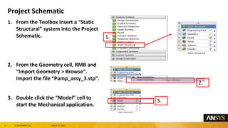
- 4. 4 ┬® 2016 ANSYS, Inc. March 11, 2016 Project Schematic 1. From the Toolbox insert a ŌĆ£Static StructuralŌĆØ system into the Project Schematic. 2. From the Geometry cell, RMB and ŌĆ£Import Geometry > BrowseŌĆØ. Import the file ŌĆ£Pump_assy_3.stpŌĆØ. 3. Double click the ŌĆ£ModelŌĆØ cell to start the Mechanical application. 1. 2. 3.
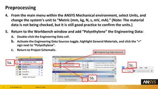
- 5. 5 ┬® 2016 ANSYS, Inc. March 11, 2016 Preprocessing 4. From the main menu within the ANSYS Mechanical environment, select Units, and change the systemŌĆÖs unit to ŌĆ£Metric (mm, kg, N, s, mV, mA).ŌĆØ (Note: The material data is not being checked, but it is still good practice to confirm the units.) 5. Return to the Workbench window and add ŌĆ£PolyethyleneŌĆØ the Engineering Data: a. Double-click the Engineering Data cell. b. Activate the Engineering Data Sources toggle, highlight General Materials, and click the ŌĆ£+ŌĆØ sign next to ŌĆ£PolyethyleneŌĆØ. c. Return to Project Schematic. 5b. 5c. 5a.
- 6. 6 ┬® 2016 ANSYS, Inc. March 11, 2016 Preprocessing 6. Refresh the Model cell: a. Click Model cell and RMB > Refresh. b. Return to the Mechanical window. 7. Change the material on the pump housing: a. Highlight ŌĆ£PumpHousingŌĆØ under geometry. b. From details change the material assignment to ŌĆ£PolyethyleneŌĆØ. 7a. 7b. 6a.
- 7. 7 ┬® 2016 ANSYS, Inc. March 11, 2016 Preprocessing 8. Change the contact behavior for one of the contact regions (shown below): a. Use the shift key to select all of the contact regions, then RMB > Rename Based on Definition. b. From the Details window, change the contact Type to ŌĆ£No SeparationŌĆØ for contact region ŌĆ£Bonded - PumpHousing to Shaft.ŌĆØ ŌĆó The remainder of the contacts will be left as ŌĆ£BondedŌĆØ (this is the default contact Type).
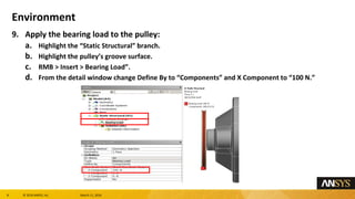
- 8. 8 ┬® 2016 ANSYS, Inc. March 11, 2016 Environment 9. Apply the bearing load to the pulley: a. Highlight the ŌĆ£Static StructuralŌĆØ branch. b. Highlight the pulleyŌĆÖs groove surface. c. RMB > Insert > Bearing LoadŌĆØ. d. From the detail window change Define By to ŌĆ£ComponentsŌĆØ and X Component to ŌĆ£100 N.ŌĆØ
- 9. 9 ┬® 2016 ANSYS, Inc. March 11, 2016 Environment 10. Apply supports to the assembly: a. Highlight the mating face on the pump housing (part 1). b. ŌĆ£RMB > Insert > Frictionless SupportŌĆØ.
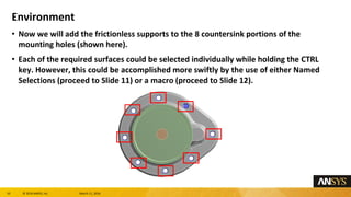
- 10. 10 ┬® 2016 ANSYS, Inc. March 11, 2016 Environment ŌĆó Now we will add the frictionless supports to the 8 countersink portions of the mounting holes (shown here). ŌĆó Each of the required surfaces could be selected individually while holding the CTRL key. However, this could be accomplished more swiftly by the use of either Named Selections (proceed to ║▌║▌▀Ż 11) or a macro (proceed to ║▌║▌▀Ż 12).
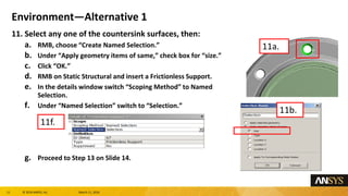
- 11. 11 ┬® 2016 ANSYS, Inc. March 11, 2016 EnvironmentŌĆöAlternative 1 11. Select any one of the countersink surfaces, then: a. RMB, choose ŌĆ£Create Named Selection.ŌĆØ b. Under ŌĆ£Apply geometry items of same,ŌĆØ check box for ŌĆ£size.ŌĆØ c. Click ŌĆ£OK.ŌĆØ d. RMB on Static Structural and insert a Frictionless Support. e. In the details window switch ŌĆ£Scoping MethodŌĆØ to Named Selection. f. Under ŌĆ£Named SelectionŌĆØ switch to ŌĆ£Selection.ŌĆØ g. Proceed to Step 13 on ║▌║▌▀Ż 14. 11a. 11b. 11f.
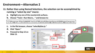
- 12. 12 ┬® 2016 ANSYS, Inc. March 11, 2016 EnvironmentŌĆöAlternative 2 11. Rather than using Named Selections, the selection can be accomplished by running a ŌĆ£select by sizeŌĆØ macro: a. Highlight any one of the countersink surfaces. b. Choose ŌĆ£Tools > Run MacroŌĆ” ŌĆØ and browse to: c. In the file browser, choose ŌĆ£selectBySize.js.ŌĆØ d. Click ŌĆ£Open.ŌĆØ e. Proceed to Step 12 on ║▌║▌▀Ż 13. 11a. 11c. 11d. C:Program FilesANSYS Incv170aisolDesignSpaceDSPagesmacros
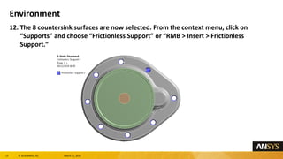
- 13. 13 ┬® 2016 ANSYS, Inc. March 11, 2016 Environment 12. The 8 countersink surfaces are now selected. From the context menu, click on ŌĆ£SupportsŌĆØ and choose ŌĆ£Frictionless SupportŌĆØ or ŌĆ£RMB > Insert > Frictionless Support.ŌĆØ
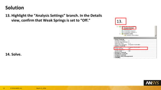
- 14. 14 ┬® 2016 ANSYS, Inc. March 11, 2016 Solution 13. Highlight the ŌĆ£Analysis SettingsŌĆØ branch. In the Details view, confirm that Weak Springs is set to ŌĆ£Off.ŌĆØ 14. Solve. 13.
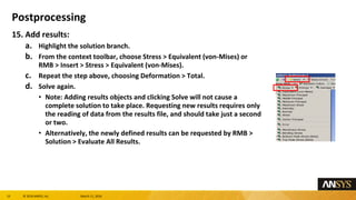
- 15. 15 ┬® 2016 ANSYS, Inc. March 11, 2016 Postprocessing 15. Add results: a. Highlight the solution branch. b. From the context toolbar, choose Stress > Equivalent (von-Mises) or RMB > Insert > Stress > Equivalent (von-Mises). c. Repeat the step above, choosing Deformation > Total. d. Solve again. ŌĆó Note: Adding results objects and clicking Solve will not cause a complete solution to take place. Requesting new results requires only the reading of data from the results file, and should take just a second or two. ŌĆó Alternatively, the newly defined results can be requested by RMB > Solution > Evaluate All Results.
- 16. 16 ┬® 2016 ANSYS, Inc. March 11, 2016 Postprocessing ŌĆó While the overall plots can be used as a reality check to verify our loads, the plots are less than ideal since much of the model is displayed in few colors. (Your results may vary slightly due to meshing differences). ŌĆó To improve the quality of results available we will ŌĆ£scopeŌĆØ results to individual parts.
- 17. 17 ┬® 2016 ANSYS, Inc. March 11, 2016 Postprocessing 16. Scope the results to specified geometry: a. Highlight the ŌĆ£SolutionŌĆØ branch and switch the selection filter to ŌĆ£BodyŌĆØ select mode. b. Select the impeller. c. ŌĆ£RMB > Insert > Stress > equivalent (von-Mises)ŌĆØ ŌĆó Notice the detail for the new result indicates a scope of 1 Body. ŌĆó Now the local variation in the results are more visually distinct. 17. Repeat the procedure above to insert ŌĆ£Total DeformationŌĆØ results for the impeller part. 18. Repeat to add individually scoped stress and deformation results for the pump housing. 16a. 16b.
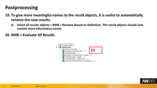
- 18. 18 ┬® 2016 ANSYS, Inc. March 11, 2016 Postprocessing 19. To give more meaningful names to the result objects, it is useful to automatically rename the new results: a. Select all results objects > RMB > Rename Based on Definition. The result objects should now contain more informative names 20. RMB > Evaluate All Results 19
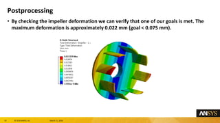
- 19. 19 ┬® 2016 ANSYS, Inc. March 11, 2016 Postprocessing ŌĆó By checking the impeller deformation we can verify that one of our goals is met. The maximum deformation is approximately 0.022 mm (goal < 0.075 mm).
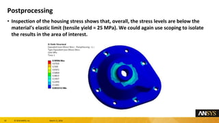
- 20. 20 ┬® 2016 ANSYS, Inc. March 11, 2016 Postprocessing ŌĆó Inspection of the housing stress shows that, overall, the stress levels are below the materialŌĆÖs elastic limit (tensile yield = 25 MPa). We could again use scoping to isolate the results in the area of interest.
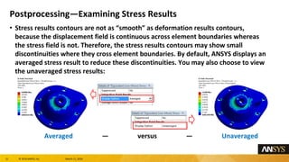
- 21. 21 ┬® 2016 ANSYS, Inc. March 11, 2016 PostprocessingŌĆöExamining Stress Results ŌĆó Stress results contours are not as ŌĆ£smoothŌĆØ as deformation results contours, because the displacement field is continuous across element boundaries whereas the stress field is not. Therefore, the stress results contours may show small discontinuities where they cross element boundaries. By default, ANSYS displays an averaged stress result to reduce these discontinuities. You may also choose to view the unaveraged stress results: Averaged ŌĆö versus ŌĆö Unaveraged
- 22. 22 ┬® 2016 ANSYS, Inc. March 11, 2016 Go Further! If you find yourself with extra time, consider the following: 1. The Mesh is very coarse. In order to get more physically meaningful results, the mesh must be refinedŌĆöapply mesh controls to refine the mesh. Try to achieve something similar to this:
- 23. 23 ┬® 2016 ANSYS, Inc. March 11, 2016 Go Further! 2. Solve again and re-examine the results:
- 24. 24 ┬® 2016 ANSYS, Inc. March 11, 2016 END Workshop 03.1: Linear Structural Analysis