New Clustering-based Forecasting Method for Disaggregated End-consumer Electricity Load Using Smart Grid Data
- 1. New Clustering-based Forecasting Method for Disaggregated End-consumer Electricity Load Using Smart Grid Data Peter Laurinec, and M├Īria Luck├Ī 14.11.2017 Slovak University of Technology in Bratislava
- 2. Motivation More accurate forecast of electricity consumption is needed due to: ŌĆó Optimization of electricity consumption. ŌĆó Distribution (utility) companies. Deregulation of the market. Purchase and sale of electricity. ŌĆó Ecological factors. However, it is very dif’¼ücult task for individual end-consumers due to: ŌĆó Stochastic behaviour (processes). ŌĆó Many factors in’¼éuencing the consumption: ŌĆó Seasonality ŌĆó Weather ŌĆó Holidays ŌĆó Market 1
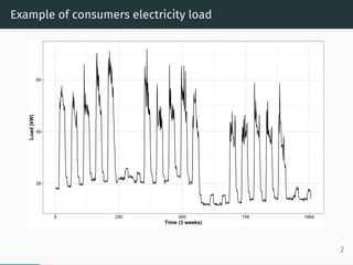
- 3. Example of consumers electricity load 20 40 60 0 250 500 750 1000 Time (3 weeks) Load(kW) 2
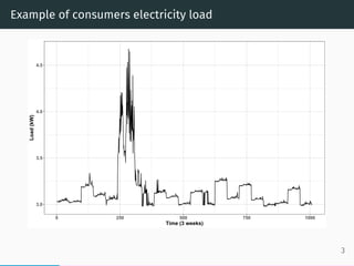
- 4. Example of consumers electricity load 3.0 3.5 4.0 4.5 0 250 500 750 1000 Time (3 weeks) Load(kW) 3
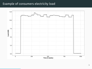
- 5. Example of consumers electricity load 0.0 2.5 5.0 7.5 10.0 12.5 0 250 500 750 1000 Time (3 weeks) Load(kW) 4
- 6. Example of consumers electricity load - residential 0 1 2 3 0 250 500 750 1000 Time (3 weeks) Load(kW) 5
- 7. Classical vs. our approach The classical way is to train a model for every consumer separately (drawbacks). Our approach uses data from all consumers in a smart grid to overcome stochastic changes and noisy character of data (time series). Solution: clustering of all consumers. 6
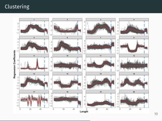
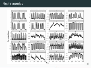
- 8. Our method We will suppose that N is a number of consumers, the length of the training set is 21 days (3 weeks) whereby in every day we will consider 24 ├Ś 2 = 48 measurements, and we will execute one hour ahead forecasts. 1. Starting with iteration iter = 0. 2. Creating of time series for each consumer of the lengths of three weeks. 3. Normalisation of each time series by z-score (keeping a mean and a standard deviation in memory for every time series). 4. Computation of representations of each time series. 5. K-means clustering of representations and an optimal number of clusters is computed. 6. The extraction of K centroids and using them as training set to any forecasting method. 7. The denormalisation of K forecasts using the stored mean and standard deviation to produce N forecasts. 8. iter = iter + 1. If iter is divisible by 24 (iter mod 24 = 0 mod 24) then steps 4) and 5) are performed otherwise they are skipped and the stored centroids are used. 7
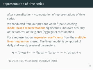
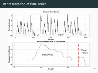
- 9. Representation of time series After normalisation -> computation of representations of time series. We conducted from our previous works 1 that clustering model-based representations signi’¼ücantly improves accuracy of the forecast of the global (aggregate) consumption. For a representation, regression coefficients from the multiple linear regression is used. The linear model is composed of daily and weekly seasonal parameters. xt = ╬▓d1utd1 + ┬Ę ┬Ę ┬Ę + ╬▓dsutds + ╬▓w1utw1 + ┬Ę ┬Ę ┬Ę + ╬▓w6utw6 + ╬Ąt 1 Laurinec et al., WCECS (2016) and ICDMW (2016) 8
- 10. Representation of time series ŌłÆ1 0 1 2 3 0 250 500 750 1000 Length NormalizedLoad Original Time Series Daily Period Weekly Period ŌłÆ1 0 1 0 20 40 Length RegressionCoefficients Final Representation of Time Series 9
- 11. Clustering 17 18 19 20 13 14 15 16 9 10 11 12 5 6 7 8 1 2 3 4 0 20 40 0 20 40 0 20 40 0 20 40 ŌłÆ1 0 1 2 3 ŌłÆ2 ŌłÆ1 0 1 2 3 ŌłÆ2 0 2 ŌłÆ2 0 2 ŌłÆ2 ŌłÆ1 0 1 2 3 ŌłÆ1 0 1 2 ŌłÆ3 ŌłÆ2 ŌłÆ1 0 1 2 ŌłÆ2 0 2 ŌłÆ2 ŌłÆ1 0 1 2 0 2 4 ŌłÆ2 0 2 4 ŌłÆ1 0 1 2 ŌłÆ2 0 2 4 ŌłÆ2 0 2 ŌłÆ2 ŌłÆ1 0 1 2 3 ŌłÆ1 0 1 2 ŌłÆ1 0 1 2 3 0 2 4 ŌłÆ2 ŌłÆ1 0 1 2 ŌłÆ2 ŌłÆ1 0 1 2 Length RegressionCoefficients 10
- 12. Final centroids 17 18 19 20 13 14 15 16 9 10 11 12 5 6 7 8 1 2 3 4 0 250 500 750 1000 0 250 500 750 1000 0 250 500 750 1000 0 250 500 750 1000 ŌłÆ0.5 0.0 0.5 1.0 1.5 ŌłÆ1.5 ŌłÆ1.0 ŌłÆ0.5 0.0 0.5 1.0 ŌłÆ0.50 ŌłÆ0.25 0.00 0.25 ŌłÆ1 0 1 ŌłÆ1.0 ŌłÆ0.5 0.0 0.5 ŌłÆ1.0 ŌłÆ0.5 0.0 0.5 1.0 ŌłÆ1.0 ŌłÆ0.5 0.0 0.5 ŌłÆ1.0 ŌłÆ0.5 0.0 0.5 1.0 ŌłÆ1.0 ŌłÆ0.5 0.0 0.5 1.0 ŌłÆ0.5 0.0 0.5 1.0 0 1 0 1 2 ŌłÆ0.5 0.0 0.5 ŌłÆ1.0 ŌłÆ0.5 0.0 0.5 1.0 ŌłÆ0.5 0.0 0.5 1.0 1.5 0 1 0 1 2 0 1 2 3 4 5 ŌłÆ1.0 ŌłÆ0.5 0.0 0.5 1.0 ŌłÆ1 0 1 Time NormalizedLoad 11
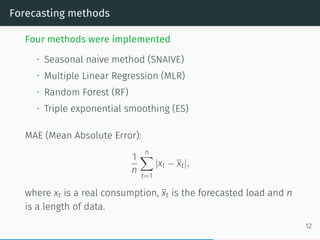
- 13. Forecasting methods Four methods were implemented ŌĆó Seasonal naive method (SNAIVE) ŌĆó Multiple Linear Regression (MLR) ŌĆó Random Forest (RF) ŌĆó Triple exponential smoothing (ES) MAE (Mean Absolute Error): 1 n nŌłæ t=1 |xt ŌłÆ xt|, where xt is a real consumption, xt is the forecasted load and n is a length of data. 12
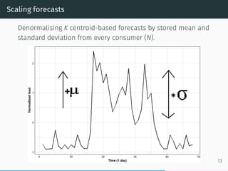
- 14. Scaling forecasts Denormalising K centroid-based forecasts by stored mean and standard deviation from every consumer (N). 13
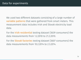
- 15. Data for experiments We used two different datasets consisting of a large number of variable patterns that were gathered from smart meters. This measurement data includes Irish and Slovak electricity load data. For the Irish residential testing dataset (3639 consumers) the data measurements from 1.2.2010 to 21.2.2010. For the Slovak factories testing dataset (3607 consumers) the data measurements from 10.2.2014 to 2.3.2014. 14
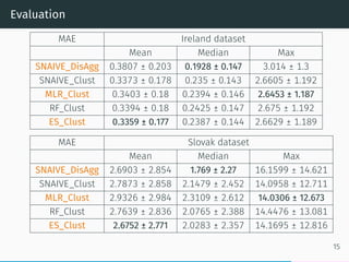
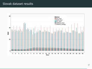
- 16. Evaluation MAE Ireland dataset Mean Median Max SNAIVE_DisAgg 0.3807 ┬▒ 0.203 0.1928 ┬▒ 0.147 3.014 ┬▒ 1.3 SNAIVE_Clust 0.3373 ┬▒ 0.178 0.235 ┬▒ 0.143 2.6605 ┬▒ 1.192 MLR_Clust 0.3403 ┬▒ 0.18 0.2394 ┬▒ 0.146 2.6453 ┬▒ 1.187 RF_Clust 0.3394 ┬▒ 0.18 0.2425 ┬▒ 0.147 2.675 ┬▒ 1.192 ES_Clust 0.3359 ┬▒ 0.177 0.2387 ┬▒ 0.144 2.6629 ┬▒ 1.189 MAE Slovak dataset Mean Median Max SNAIVE_DisAgg 2.6903 ┬▒ 2.854 1.769 ┬▒ 2.27 16.1599 ┬▒ 14.621 SNAIVE_Clust 2.7873 ┬▒ 2.858 2.1479 ┬▒ 2.452 14.0958 ┬▒ 12.711 MLR_Clust 2.9326 ┬▒ 2.984 2.3109 ┬▒ 2.612 14.0306 ┬▒ 12.673 RF_Clust 2.7639 ┬▒ 2.836 2.0765 ┬▒ 2.388 14.4476 ┬▒ 13.081 ES_Clust 2.6752 ┬▒ 2.771 2.0283 ┬▒ 2.357 14.1695 ┬▒ 12.816 15
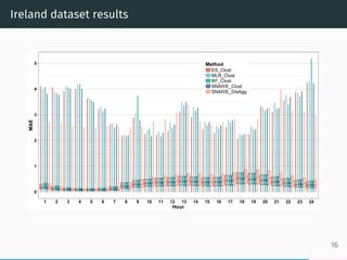
- 17. Ireland dataset results 0 1 2 3 4 5 1 2 3 4 5 6 7 8 9 10 11 12 13 14 15 16 17 18 19 20 21 22 23 24 Hour MAE Method ES_Clust MLR_Clust RF_Clust SNAIVE_Clust SNAIVE_DisAgg 16
- 18. Slovak dataset results 0 20 40 60 1 2 3 4 5 6 7 8 9 10 11 12 13 14 15 16 17 18 19 20 21 22 23 24 Hour MAE Method ES_Clust MLR_Clust RF_Clust SNAIVE_Clust SNAIVE_DisAgg 17
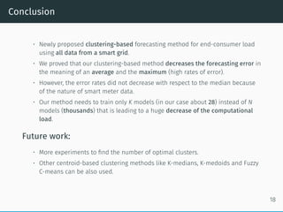
- 19. Conclusion ŌĆó Newly proposed clustering-based forecasting method for end-consumer load using all data from a smart grid. ŌĆó We proved that our clustering-based method decreases the forecasting error in the meaning of an average and the maximum (high rates of error). ŌĆó However, the error rates did not decrease with respect to the median because of the nature of smart meter data. ŌĆó Our method needs to train only K models (in our case about 28) instead of N models (thousands) that is leading to a huge decrease of the computational load. Future work: ŌĆó More experiments to ’¼ünd the number of optimal clusters. ŌĆó Other centroid-based clustering methods like K-medians, K-medoids and Fuzzy C-means can be also used. 18
