On Estimation of Surface Soil Moisture.ppt
ŌĆóDownload as PPT, PDFŌĆó
0 likesŌĆó7 views

On Estimation of Surface Soil Moisture


On Estimation of Surface Soil Moisture.ppt
- 1. On Estimation of Soil Moisture with SAR Jiancheng Shi ICESS University of California, Santa Barbara
- 2. Importance of Water Circle
- 3. Basic Consideration (1) Common idea of the current algorithm ŌĆó ŌĆó Inverse - two equations ’ā× two unknowns. It can be re-ranged to one equation for one unknown. Disadvantages: ŌĆó Requires both formula all in good accuracy ŌĆó Error in the estimated one unknown’ā× the other ) , , ( ) ( 2 1 r r pp s or s f f ’āŚ ’ĆĮ ’üź ’ü│
- 4. Basic Consideration (1) - continue ) log( 36 . 3 ) log( 09 . 3 ) log( ) log( 78 . 4 ) log( 79 . 3 19 . 2 ) ) ( log( ) log( 57 . 2 ) log( 09 . 2 03 . 2 ) log( 2 hh vv h hh vv r hh vv R W ks S ks ’ü│ ’ü│ ’ü│ ’ü│ ’ü│ ’ü│ ’ĆŁ ’Ć½ ’ĆŁ ’ĆĮ ’Ć½ ’ĆŁ ’ĆĮ ’ĆĮ ’Ć½ ’ĆŁ ’ĆĮ in (a) in (b) in (c) ŌĆó Different weight ’ā× sensitive to different surface parameter ŌĆó Independent direct estimation of soil moisture and RMS height (a) ks (b) Sr (c) Rh
- 5. Basic Consideration (2) IEM -- Power expansion and nonlinear relationships ’üø ’üØ ! ) 0 , 2 ( | | 2 exp 2 1 2 2 2 2 2 n k W I s s k k x n n n pp n z o pp ’ĆŁ ’ĆŁ ’ĆĮ ’āź ’éź ’ĆĮ ’ü│ Higher order inverse formula ’ā× improve accuracy Example: estimate surface RMS height 28 . 0 ) , ( ) 2 ( ’ĆĮ RMSE f hh vv ’ü│ ’ü│ 36 . 0 ) , ( ) 1 ( ’ĆĮ RMSE f hh vv ’ü│ ’ü│ s s sŌĆÖ sŌĆÖ
- 6. Basic Consideration (3) Polorization Magnitude Roughness function SP PO GO Tradition Backscattering Models ’üø ’üØ 2 2 2 ) sin ( exp ) ( ) ( ’ü▒ kl kl ks ’ĆŁ ’ü▒ ’üź ’ü▒ ’üź ’ü▒ ’üź ’ü▒ ’üź 2 2 sin cos sin cos ’ĆŁ ’Ć½ ’ĆŁ ’ĆŁ r r r r ) 1 ( ) 1 ( r r ’üź ’üź ’Ć½ ’ĆŁ ) 2 tan exp( 2 1 2 m m ’ü▒ ’ĆŁ ’üø ’üØ ’ā║ ’ā╗ ’ā╣ ’ā¬ ’ā½ ’ā® ’ĆŁ ’āź ’āŚ ’ĆŁ ’éź ’ĆĮ n kl n n kl kl kl n n 4 ) ( exp ! ) cos ( ) sin ( exp ) ( 2 1 2 2 ’ü▒ ’ü▒ ’Ć© ’Ć® ’üø ’üØ ’Ć© ’Ć®2 2 2 2 sin cos sin 1 sin ) 1 ( ’ü▒ ’üź ’ü▒ ’üź ’ü▒ ’üź ’ü▒ ’üź ’ĆŁ ’Ć½ ’Ć½ ’ĆŁ ’ĆŁ r r r r ŌĆó Inverse model for different roughness region ’ā× improve accuracy
- 7. Validation Using Michigan's Scatterometer Data ’éĘ Correlation: mv - 0.75, rms height - 0.96 ’éĘ RMSE: mv - 4.1%, rms height - 0.34cm mv S RMSE for S Measured parameters Estimated incidence
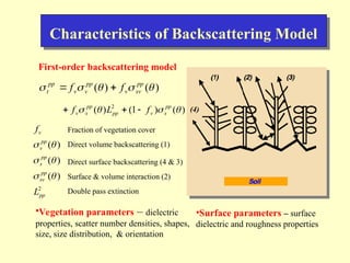
- 8. Characteristics of Backscattering Model (4) ) ( ) ( ’ü▒ ’ü│ ’ü▒ ’ü│ ’ü│ pp sv v pp v v pp t f f ’Ć½ ’ĆĮ ) ( ) 1 ( ) ( 2 ’ü▒ ’ü│ ’ü▒ ’ü│ pp s v pp pp s v f L f ’ĆŁ ’Ć½ ’Ć½ First-order backscattering model ŌĆóSurface parameters ŌĆō surface dielectric and roughness properties ŌĆóVegetation parameters ŌĆō dielectric properties, scatter number densities, shapes, size, size distribution, & orientation 2 ) ( ) ( ) ( pp pp sv pp s pp v v L f ’ü▒ ’ü│ ’ü▒ ’ü│ ’ü▒ ’ü│ Fraction of vegetation cover Direct volume backscattering (1) Direct surface backscattering (4 & 3) Surface & volume interaction (2) Double pass extinction
- 9. Radar Target Decomposition Covariance (or correlation) matrix ’üø ’üØ ’ā║ ’ā║ ’ā╗ ’ā╣ ’ā¬ ’ā¬ ’ā½ ’ā® ’ĆĮ ’ü║ ’ü▓ ’ü© ’ü▓ 0 0 0 0 1 * c T Decomposition based on eigenvalues and eigenvectors ’üø ’üØ ' 3 3 1 ' 2 2 1 ' 1 1 1 k k k k k k T ’éĘ ’Ć½ ’éĘ ’Ć½ ’éĘ ’ĆĮ ’ü¼ ’ü¼ ’ü¼ where, ’ü¼ are the eigenvalues of the covariance matrix, k are the eigenvectors, and kŌĆÖ means the adjoint (complex conjugate transposed ) of k. * hh hh S S c ’ĆĮ * * hh hh vv hh S S S S ’ĆĮ ’ü▓ * * 2 hh hh hv hv S S S S ’ĆĮ ’ü© * * hh hh vv vv S S S S and ’ĆĮ ’ü║
- 10. Radar Target Decomposition Technique Total Power: single, double, multi VV: single, double, multi HH Correlation or covariance matrix -> Eigen values & vectors T T T * 3 3 3 * 2 2 2 * 1 1 1 K K K K K K T ’ü¼ ’ü¼ ’ü¼ ’Ć½ ’Ć½ ’ĆĮ VV, HH, VH
- 11. Relationships in scattering components between decomposition and backscattering model 1. First component in decomposition (single scattering) ŌĆō direct volume, surface & its passes vegetation 2. Second component (double-bounce scattering) ŌĆō Surface & volume interaction terms 3. Third component ŌĆō defuse or multi-scattering terms
- 12. Properties of Double Scattering Component under Time Series Measurements 1. Variation in Time Scale ŌĆó surface roughness ŌĆó vegetation growth ŌĆó surface soil moisture 2. In backscattering Model 3. Ratio of two measurements ŌĆó independent of vegetation properties ŌĆó depends only on the reflectivity ratio ) ( ) ( ) ( 2 ) ( 2 ’ü▒ ’ü▒ ’ü½ ’ü▒ ’ü▒ ’ü│ pp pp s pp pp sv dL R ’ĆĮ n pp m pp n pp m pp R R ’ĆŁ ’ĆŁ ’ĆŁ ’ĆŁ ’ĆĮ 2 2 ’ü│ ’ü│
- 13. Comparison with Field Measurements VV, HH, VH Two Corn Fields Dielectric Constant Date n hh n vv m hh m vv R R R R ’ĆŁ ’ĆŁ ’ĆŁ ’ĆŁ n hh n vv m hh m vv ’ĆŁ ’ĆŁ ’ĆŁ ’ĆŁ 2 2 2 2 ’ü│ ’ü│ ’ü│ ’ü│ ’āø ’ĆŁ ’ĆŁ ’ĆŁ ’ĆŁ n hh n vv m hh m vv 2 2 2 2 ’ü│ ’ü│ ’ü│ ’ü│ Normalized VV & HH cross product of double scattering components for any n < m Corresponding reflectivity ratio ’āø ’ĆŁ ’ĆŁ ’ĆŁ ’ĆŁ n hh n vv m hh m vv R R R R Correlation=0.93, RMSE=0.42 dB
- 14. Estimate Absolute Surface Reflectance A) B) C) 2 2 | | | | m vv n vv v nm A ’üĪ ’üĪ ’ĆĮ 2 2 | | | | m hh n hh h nm A ’üĪ ’üĪ ’ĆĮ m hh n hh m vv n vv c nm A | | | | | | | | ’üĪ ’üĪ ’üĪ ’üĪ ’éĘ ’ĆĮ ) ( c nm v nm A f A ’ĆĮ ) ( c nm h nm A f A ’ĆĮ ’āĘ ’āĘ ’āĖ ’āČ ’ā¦ ’ā¦ ’ā© ’ā” ’ĆŁ ’éĘ ’ĆĮ ’ĆŁ 2 2 2 2 2 | | | | 1 | | | | | | m hh n hh n hh m hh n hh ’üĪ ’üĪ ’üĪ ’üĪ ’üĪ h nm m hh n hh n hh A ’ĆŁ ’ĆŁ ’ĆĮ 1 | | | | | | 2 2 2 ’üĪ ’üĪ ’üĪ ’āĘ ’āĘ ’āĖ ’āČ ’ā¦ ’ā¦ ’ā© ’ā” ’Ć½ ’ĆŁ ’é╗ ’ĆŁ h nm v nm h nm v nm m hh n hh A A A A f 2 2 | | | | ’üĪ ’üĪ A) ) log( ) log( c nm v nm A A ’é╗ B) C) estimation
- 15. Current Evaluations ŌĆó Validity range of the second component measurements ŌĆō Effect of radar calibration and system noise ŌĆō What type and vegetation condition? ŌĆó How to obtain vegetation and surface roughness information ŌĆō What we can do with the first component measurements? ŌĆó What to do with sparse vegetated surface?
- 16. Summary ŌĆó Time series measurements with second decomposed components (double reflection) ŌĆō A promising (direct and simple technique) to estimate the relative change in dielectric constant for certain type of the vegetated surfaces ŌĆō A great possibility to derive soil moisture algorithm for the vegetated surface ŌĆó Advantages of this technique ŌĆō Do not require any information on vegetation ŌĆō Can be applied to partially covered vegetation surface