Predict Backorder on a supply chain data for an Organization
ŌĆóDownload as PPTX, PDFŌĆó
1 likeŌĆó1,462 views

The document discusses predicting backorders using supply chain data. It defines backorders as customer orders that cannot be filled immediately but the customer is willing to wait. The data analyzed consists of 23 attributes related to a garment supply chain, including inventory levels, forecast sales, and supplier performance metrics. Various machine learning algorithms are applied and evaluated on their ability to predict backorders, including naive Bayes, random forest, k-NN, neural networks, and support vector machines. Random forest achieved the best accuracy of 89.53% at predicting backorders. Feature selection and data balancing techniques are suggested to potentially further improve prediction performance.


![Gamma
The gamma parameter defines how far the
influence of a single training example reaches,
with low values meaning ŌĆśfarŌĆÖ and
high values meaning ŌĆścloseŌĆÖ.
Kernel
A powerful insight is that the linear SVM can be
rephrased using the inner product of any
two given observations, rather than
the observations themselves. The inner product between
two vectors is the sum of the multiplication of each pair of input
values
The inner product of the vectors [2, 3] and [5, 6] is 2*5 + 3*6
or 28
Radial Kernel SVM (Radial basis function)
K(x,xi) = exp(-gamma * sum((x ŌĆō xi^2))
Where gamma is a parameter that must be specified to the learning algorithm. A good default value for gamma is 0.1, where gamma
is often 0 < gamma < 1. The radial kernel is very local and can create complex regions within the feature space, like closed polygons
in two-dimensional space.](https://image.slidesharecdn.com/cs513predictbackorderfinalpresentation-180219180909/85/Predict-Backorder-on-a-supply-chain-data-for-an-Organization-31-320.jpg)


Predict Backorder on a supply chain data for an Organization
- 1. CAN WE PREDICT BACKORDER? (Supply Chain Data) Salil Chawla, Atharva Nandurdikar , Piyush Srivastava, Anil Thadani, Siddharaj Deshmukh
- 2. WHAT IS BACKORDER? ŌĆó Sometimes when a company makes an order for a good, a company or store may have run out of stock in its inventory. A company who has run out of the demanded product but has re-ordered the goods would promise its customers that it would ship the goods when they become available. A customer who is willing to wait for some time until the company has restocked the merchandise, would have to place a back order. A back order only exists if customers are willing to wait for the order. ŌĆó A customer order that cannot be filled when presented, and for which the customer is prepared to wait for some time. The percentage of items backordered and the number of backorder days are important measures of the quality of a company's customer service and the effectiveness of its inventory management.
- 3. ABOUT DATA ŌĆó We have selected the data of (Global Garment Supply Chain Data) from datahub ŌĆó In total, it consists 23 attributes out of which 6 are binary, 1 notation and the other 16 are numeric. ŌĆó Among the attributes, some represents the status of transiting, like: lead time of the product (lead-time, as weeks) and amount of product in transit from source (in transit qty, units). ŌĆó This data represents product supplierŌĆÖs historical performance. Some suppliers have not been scored and have a dummy value of -99 loaded. ŌĆó brief explanation and data types of the 23 attributes
- 4. ATTRIBUTES
- 5. DATA ISSUES ŌĆó Knowing from the data,1% of the products actually went on backorder, which creates a big imbalance on the classes. ŌĆó It is a common problem for a real dataset. ŌĆó Preferably, it is required that a classifier provides a balanced degree of predictive accuracy for both the minority and majority classes on the dataset. However, in many standard learning algorithms, it is found that classifiers tend to provide a severely imbalanced degree of accuracy
- 7. First few rows (not normalized but NA values filled Using KNN) Mention: Assumption is that min and max values are the only ones possible and hence used that for normalization.
- 9. Variable selection ’é¦ After cleaning the data, we started applying the models on different combination of variables. ’é¦ Accuracy of KNN model when applied over all the variables was 77%. ’é¦ Need to select particular combination of variables for better accuracy. ’é¦ Variable selection technique is very effective technique to fetch best set of variables for a model. ’é¦ First step is to check which variables are ŌĆścorrelatedŌĆÖ.
- 11. Findings of Correlation ŌĆó The dark Blue circles forming a diagonal line show that, a variable is highly correlated with itself. ŌĆó However, there is high correlation between two sets containing three variables each viz. forecast_3, 6 & 9_months and sales_1, 3,6,& 9_month. ŌĆó Choosing one variable from each of these sets will reduce multi-correlation and in turn increase the accuracy of model. ŌĆó If there are K potential Independent Variables, there are 2k distinct subsets to be tasted. ŌĆó How to choose best set of variables for a model? ŌĆó What are different techniques for variable selection? To be continuedŌĆ”
- 12. C 5.0 for Variable Selection ŌĆó C 5.0 was Implemented over complete dataset to analyze decision trees. ŌĆó It measured predictor importance by determining the percentage of training set samples that fall into all the terminal nodes after the split. ŌĆó First two predictors ŌĆśnational_invŌĆÖ ŌĆśforecast_3_monthŌĆÖ in the first split automatically bears 100% importance. ŌĆó Based on the best ŌĆścategoryŌĆÖ contained in an attribute, other variables are ranked as shown in adjoining figure.
- 13. Random Forest for Variable Selection ŌĆó To get better accuracy, we applied random forest which decorrelated 200 trees (classifiers) generated on different bootstrapped samples from Training data. ŌĆó Averaging the trees helped us to reduce ŌĆśvarianceŌĆÖ & avoid ŌĆśoverfittingŌĆÖ. ŌĆó The out of bag estimate was calculated to find mean prediction error on each training sample. ŌĆó The graph shows attributes in decreasing order of ŌĆśMean decrease accuracyŌĆÖ. ŌĆó Hence final variable set selected for all further models is: ŌĆó 'national_inv', 'in_transit_qty', 'lead_time', 'forecast_3_month', 'sales_1_month', 'min_bankŌĆÖ, 'perf_6_month_avgŌĆÖ,'local_bo_qty','stop_auto_byŌĆÖ, ŌĆÖdeck_risk','went_on_backorder'
- 14. Naive Bayes ’é¦ It calculates the posterior probability for each class. ’é¦ The class with the highest posterior probability is the outcome of prediction. Assumption: It works based on the frequency count of each variable, so variables are independent of each other. P(c|x) is the posterior probability of class (c, target) given predictor (x, attributes). P(c) is the prior probability of class. P(x|c) is the likelihood which is the probability of predictor given class. P(x) is the prior probability of predictor.
- 15. Naïve Bayes Result Confusion Matrix: Accuracy : Highly Imbalanced Dataset Balanced Dataset
- 16. Random Forest ’üĄ First applied on Highly Imbalanced data and then tried to Balanced it. Results on Highly Imbalanced data: ’üĄ Used Random Forest because it performs well on classification model, and it doesnŌĆÖt require data to be normalized, correlation doesnŌĆÖt matter and works on binary split like decision tree. ’üĄ We have tried to overcome the overfitting if any.
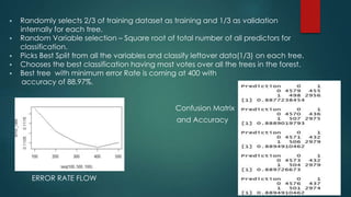
- 17. ’é¦ Randomly selects 2/3 of training dataset as training and 1/3 as validation internally for each tree. ’é¦ Random Variable selection ŌĆō Square root of total number of all predictors for classification. ’é¦ Picks Best Split from all the variables and classify leftover data(1/3) on each tree. ’é¦ Chooses the best classification having most votes over all the trees in the forest. ’é¦ Best tree with minimum error Rate is coming at 400 with accuracy of 88.97%. Confusion Matrix and Accuracy ERROR RATE FLOW
- 18. Tuned Random Forest ŌĆó We tried to find the optimal mtry and ntree where the out of bag error rate stabilizes and reach minimum. ŌĆó We got at ntree=500, mtry=6
- 19. Applying Un-weighted kNN model (81.6%)
- 20. Applying Weighted kNN model (84.2%)
- 21. kNN Contd..
- 22. Applying Neural Network model ’üĄ Although it is not mandatory to normalize the data, normalizing helps the algorithm reach global minima with higher probability. ’üĄ Due to lack of convergence for neurons 3 and further we increased stepmax and threshold values.
- 23. Accuracy of Neural Network (47-50%) ’üĄ Optimal no. of hidden layers were found to be 2 ’üĄ Trying with un-normalized values made little change in the results ŌĆō accuracy decreased.
- 24. Values of neurons: Graph of Accuracy
- 26. Why clustering may not be good for our data!!
- 28. What is Support Vector Machine ? Support Vector MachineŌĆØ (SVM) is a supervised machine learning algorithm which can be used for both classification or regression challenges. However, it is mostly used in classification problems. In this algorithm, we plot each data item as a point in n-dimensional space (where n is number of features you have) with the value of each feature being the value of a particular coordinate. Then, we perform classification by finding the hyper-plane that differentiate the two classes very well.
- 29. Maximal-Margin Classifier (hypothetical classifier) The numeric input variables (x) in your data (the columns) form an n-dimensional space. For example, if you had two input variables, this would form a two-dimensional space. B0 + (B1 * X1) + (B2 * X2) = 0 Where the coefficients (B1 and B2) that determine the slope of the line and the intercept (B0) are found by the learning algorithm, and X1 and X2 are the two input variables. The distance between the line and the closest data points is referred to as the margin These points are called the support vectors. They support or define the hyperplane. By plugging in input values into the line equation, you can calculate whether a new point is above or below the line. Above the line, the equation returns a value greater than 0 and the point belongs to the first class (class 0). Below the line, the equation returns a value less than 0 and the point belongs to the second class (class 1). A value close to the line returns a value close to zero and the point may be difficult to classify.
- 30. Soft Margin Classifier / Regularization parameter This change allows some points in the training data to violate the separating line. The C parameters defines the amount of violation of the margin allowed. During the learning of the hyperplane from data, all training instances that lie within the distance of the margin will affect the placement of the hyperplane and are referred to as support vectors. And as C affects the number of instances that are allowed to fall within the margin, C influences the number of support vectors used by the model. The smaller the value of C, the more sensitive the algorithm is to the training data (higher variance and lower bias). a very small value of C will cause the optimizer to look for a larger-margin separating hyperplane, even if that hyperplane misclassifies more points. The larger the value of C, the less sensitive the algorithm is to the training data (lower variance and higher bias). Large values of C, the optimization will choose a smaller-margin hyperplane if that hyperplane does a better job of getting all the training points classified correctly.
- 31. Gamma The gamma parameter defines how far the influence of a single training example reaches, with low values meaning ŌĆśfarŌĆÖ and high values meaning ŌĆścloseŌĆÖ. Kernel A powerful insight is that the linear SVM can be rephrased using the inner product of any two given observations, rather than the observations themselves. The inner product between two vectors is the sum of the multiplication of each pair of input values The inner product of the vectors [2, 3] and [5, 6] is 2*5 + 3*6 or 28 Radial Kernel SVM (Radial basis function) K(x,xi) = exp(-gamma * sum((x ŌĆō xi^2)) Where gamma is a parameter that must be specified to the learning algorithm. A good default value for gamma is 0.1, where gamma is often 0 < gamma < 1. The radial kernel is very local and can create complex regions within the feature space, like closed polygons in two-dimensional space.
- 32. Data Preparation for SVM How to best prepare training data when learning an SVM model. Numerical Inputs: SVM assumes that our inputs are numeric. If we have categorical inputs we may need to covert them to binary dummy variables (one variable for each category). Binary Classification: Basic SVM is intended for binary (two-class) classification problems. Although, extensions have been developed for regression and multi-class classification. R package : e1071 package
- 33. Business Recommendations: National Inventory ŌĆō Define min and max quantity levels at the national Inventory level. In Transit Quantity ŌĆō Keep a track of amount of the product in transit from the source, as delaying this would affect the business negatively. Lead Time ŌĆō Transit time required from the source needs to known well in advance, and guaranteed. Forecast 3 Months ŌĆō Forecast Sales for the next 3 months of the product this will help to avoid the product from going on backorder. Sales 1 Month ŌĆō Sales quantity for the prior 1 month gives us a good guess that how much quantity would be expected in the current month. Min_bank ŌĆō A minimum recommended amount of stock needs to be defined. Perf_6_moth_avg ŌĆō Source performance for prior 6 month period from which the quantity is manufactured or is to be brought is to be considered to avoid backordering. Local back Order Quantity: Quantity of the particular product that went on backorder in local markets should be studied. Stop Auto buy : Auto buying of products needs to be kept in check, keeping inventory in perspective. Deck Risk : The product lying on deck (in shop, in ship containers) needs to be considered.
- 34. Algorithm Accuracy on Imbalanced dataset Accuracy on Balanced Dataset Naïve Bayes 16.3% 43.4% Random Forest 98.9% 89.5% kNN unweighted 98.9% 81.6% Knn weighted 98.9 84.2% Neural Network 13.4% 48% SVM 62% 65% Algorithm Summary
- 35. Conclusion ’üĄ Compared the accuracy of each algorithm ’üĄ Random forest was the best algorithm with an accuracy of 89.53%. ’üĄ More feature engineering or data balancing probably could have resulted in better accuracies.
- 36. Reference ’é┐ http://www.listendata.com/2014/11/random-forest-with-r.html ’é┐ http://projekter.aau.dk/projekter/files/262657498/master_thesis.pdf ’é┐ https://old.datahub.io/dataset/global-garment-supply-chain-data