�ݺ�ߣ

Robust Design and Variation
Reduction Using DiscoverSim™
John Noguera
CTO & Co-Founder
SigmaXL, Inc.
www.SigmaXL.com
September 24, 2012

Copyright © 2012, SigmaXL, Inc.

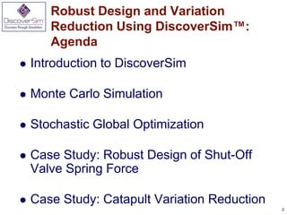
Reduction Using DiscoverSim™:
Agenda
 Introduction to DiscoverSim

 Monte Carlo Simulation

 Stochastic Global Optimization

 Case Study: Robust Design of Shut-Off
Valve Spring Force

 Case Study: Catapult Variation Reduction
2

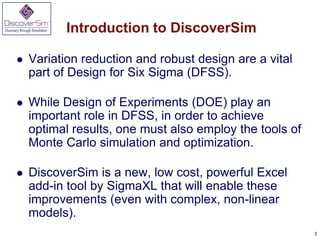
Introduction to DiscoverSim

 Variation reduction and robust design are a vital
part of Design for Six Sigma (DFSS).

 While Design of Experiments (DOE) play an
important role in DFSS, in order to achieve
optimal results, one must also employ the tools of
Monte Carlo simulation and optimization.

 DiscoverSim is a new, low cost, powerful Excel
add-in tool by SigmaXL that will enable these
improvements (even with complex, non-linear
models).
3


4

 Stochastic Global Optimization can be achieved using a
hybrid methodology of Dividing Rectangles (DIRECT),
Genetic Algorithm, and Sequential Quadratic
Programming.

 Simulation and optimization speed are realized using
DiscoverSim's Excel Formula Interpreter.
 Utilizes Gauss Engine by Aptech.
 Common Object Interface (COI) by Econotron Software to
implement an Excel spreadsheet in Gauss Engine.
 The Gauss Random Number Generator is the “KISS+Monster”
random number generator developed by George Marsaglia. This
algorithm produces random integers between 0 and 232 – 1 and
has a period of 108859.

5

Distributions in DiscoverSim

6

Monte Carlo Simulation
We start with the Y = f(X) Model, also
known as the “Transfer Function”:

X Process Y

 The Y = f(X) model should be based on theory, process knowledge, or
the prediction formula of a designed experiment or regression
analysis.
 This prediction equation should be validated prior to use in
DiscoverSim: “All models are wrong, some are useful” – George Box.
 The results of any Monte Carlo Simulation/Optimization should also be
validated with further experimentation or use of prototypes.
7

 After the Y = f(X) relationship has been validated, an important
question that then needs to be answered is: “What does the
distribution of Y look like when I cannot hold X constant, but have
some uncertainty in X?” In other words, “How can I quantify my risk?”.

 Monte Carlo simulation comes in to solve the complex problem of
dealing with uncertainty by “brute force” using computational power.

 The Monte Carlo method was coined in the
1940s by John von Neumann, Stanislaw Ulam
and Nicholas Metropolis, while they were
working on nuclear weapon projects in the Los
Alamos National Laboratory. It was named in
homage to Monte Carlo casino, a famous
casino, where Ulam's uncle would often
gamble away his money.
8

The following diagram illustrates a simple Monte Carlo simulation using
DiscoverSim with three different input distributions (X’s also known as
“Assumptions”)

Y = A1 + A2 + A3
10,000 Replications

A random draw is performed from each input distribution, Y is
calculated, and the process is repeated 10,000 times. The
histogram and descriptive statistics show the simulation results.
9

Selecting a Distribution

 Selecting the correct distribution is a critical step towards
building a useful model.

 The best choice for a distribution is one based on known
theory, for example the use of a Weibull Distribution for
reliability modeling.

 A common distribution choice is the Normal Distribution,
but this assumption should be verified with data that
passes a normality test with a minimum sample size of 30;
preferably 100.

10


 If data is available and the distribution is not normal, use
DiscoverSim’s Distribution Fitting tool to find a best fit
distribution.

 Alternatively, the Pearson Family Distribution allows you to
simply specify Mean, StdDev, Skewness and Kurtosis.

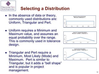
11

 In the absence of data or theory,
commonly used distributions are:
Uniform, Triangular and Pert.

 Uniform requires a Minimum and
Maximum value, and assumes an
equal probability over the range.
This is commonly used in tolerance
design.

 Triangular and Pert require a
Minimum, Most Likely (Mode) and
Maximum. Pert is similar to
Triangular, but it adds a “bell shape”
and is popular in project
management. 12

Specifying Correlations
 DiscoverSim allows you to specify correlations between
any inputs. DiscoverSim utilizes correlation copulas to
achieve the desired Spearman Rank correlation values.

 The following surface plot illustrates how a correlation
copula results in a change in the shape of a bivariate (2
input) normal distribution:

13

Optimization:
Stochastic Versus Deterministic
 Monte-Carlo simulation enables you to quantify risk,
whereas stochastic optimization enables you to minimize
risk.
 Deterministic optimization is a commonly used tool to find
a minimum or maximum (e.g., Excel Solver) but it does not
take uncertainty into account.
 Stochastic optimization will not only find the optimum X
settings that result in the best mean Y value, it will also
look for a solution that will reduce the standard deviation.
 Stochastic optimization looks for a minimum or maximum
that is robust to variation in X, thus reducing the
transmitted variation in Y. This is referred to as “Robust
Parameter Design” in DFSS.

14

Optimization: Robust Parameter
Design – Catapult Example

15

Optimization: Local Versus Global
The following surface plot illustrates a function with local
minima and a global minimum:

16


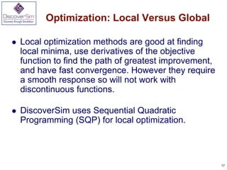
 Local optimization methods are good at finding
local minima, use derivatives of the objective
function to find the path of greatest improvement,
and have fast convergence. However they require
a smooth response so will not work with
discontinuous functions.

 DiscoverSim uses Sequential Quadratic
Programming (SQP) for local optimization.

17


 Global optimization finds the global minimum, and is
derivative free, so will work with discontinuous functions.
However because of the larger design space,
convergence is much slower than that of local
optimization.

 DiscoverSim uses DIRECT (Dividing Rectangles) and
Genetic Algorithm (GA) for global optimization.

 A hybrid of the above methodologies is also available
starting with DIRECT to do a thorough initial search,
followed by GA, and then fine tuning with SQP.

18

Hiwa, S., T. Hiroyasu and M. Miki. “Hybrid Optimization
Using DIRECT, GA, and SQP for Global Exploration”,
Doshisha University, Kyoto, Japan.
19

DiscoverSim
Components of Optimization
 Input Control: The permissible range for the control is
specified, and the control, which unlike an input
distribution, has no statistical variation.
 Think of this as a control knob like temperature.
 This is also known as a “Decision Variable”.
 An input control can be referenced by a constraint and/or an output
function.
 It is possible to have a model that consists solely of controls with
no input distributions. (In this case, the optimization is deterministic,
so the number of replications, n, should be set to 1.)
 An input control can be continuous or discrete integer.

20

DiscoverSim
Components of Optimization
 Constraint: A constraint can only be applied to an Input
Control or calculation based on Input Control:
 A constraint cannot reference an Input Distribution or Output
Response. (Constraints for Outputs, also known as Requirements,
will be added in Version 2.)
 A constraint cannot be a part of the model equation (i.e., an output
cannot reference a constraint).
 Constraints can be simple linear or complex nonlinear.
 Each constraint will contain a function of Input Controls or
Parameter Monitors on the Left Hand Side (LHS), and a constant
on the Right Hand Side (RHS).

21

DiscoverSim Optimization Metrics
Optimization Goal: Minimize Maximize

Multiple Output Weighted Sum Deviation from Target Weighted Sum Desirability

Metric:

Statistic: Mean Mean Mean Mean

Median Median
1st quartile 1st quartile

3rd quartile 3rd quartile

Minimum Minimum

Maximum Maximum

Standard Deviation Standard Deviation

Mean Squared Error: Skewness

(Taguchi Loss Function) Kurtosis
Skewness Range

Kurtosis IQR (75-25)

Range Span (95-5)

IQR (75-25) Pp
Non-Normal
Span (95-5) Ppu
Capability
Actual DPM: Ppl
Indices and
(defects per million) Ppk
Actual DPM
Calculated DPM : Cpm

(defects per million assuming %Pp (Percentile Pp)
require a
normal distribution) %Ppu (Percentile Ppu)
minimum of
%Ppl (Percentile Ppl)
10,000
%Ppk (Percentile Ppk) replications.

Case Study: Robust New Product
Design - Optimizing Shutoff Valve
Spring Force
This is an example of DiscoverSim stochastic optimization for
robust new product design, adapted from:
 Sleeper, Andrew (2006), Design for Six Sigma Statistics:
59 Tools for Diagnosing and Solving Problems in DFSS
Initiatives, NY, McGraw-Hill, pp. 782-789.
 Sleeper, Andrew, “Accelerating Product Development with
Simulation and Stochastic Optimization”,
http://www.successfulstatistics.com/
 This example is used with permission of the author.

23

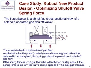
Case Study: Robust New Product
Design - Optimizing Shutoff Valve
Spring Force
The figure below is a simplified cross-sectional view of a
solenoid-operated gas shutoff valve:

The arrows indicate the direction of gas flow.
A solenoid holds the plate (shaded) open when energized. When the
solenoid is not energized, the spring pushes the plate down to shut off
gas flow.
If the spring force is too high, the valve will not open or stay open. If the
spring force is too low, the valve can be opened by the inlet gas pressure. 24

Optimizing Shutoff Valve Spring
Force
The method of specifying and testing the spring is shown
below:

The spring force requirement is 22 +/- 2 Newtons.
The spring force equation, or Y = f(X) transfer function, is calculated as
follows:
Spring Length, L = -X1 + X2 - X3 + X4
Spring Rate, R = (X8 - X7)/X6
Spring Force, Y = X7 + R * (X5 - L)
25

Case Study: Catapult Variation
Reduction
This is an example of DiscoverSim stochastic optimization for
catapult distance variation reduction, adapted from:
 John O'Neill, Sigma Quality Management,
www.sixsigmanagement.com.
 This example is used with permission of the author.

kx2
y sin  cos 
mg

26

Recommended Reading

1. Savage, Sam (2009), The Flaw of Averages:
Why We Underestimate Risk in the Face of
Uncertainty, Hoboken, NJ, Wiley.

2. Sleeper, Andrew (2006), Design for Six Sigma
Statistics: 59 Tools for Diagnosing and Solving
Problems in DFSS Initiatives, NY, McGraw-Hill.

27

Reduction Using DiscoverSim™

Questions?

�ݺ�ߣ

Robust Design And Variation Reduction Using DiscoverSim

More Related Content

Robust Design And Variation Reduction Using DiscoverSim