Sampling theorem
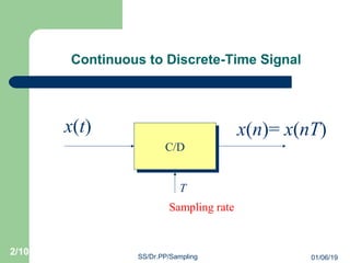
- 2. Continuous to Discrete-Time Signal C/DC/D T x(t) x(n)= x(nT) Sampling rate 01/06/19 2/10 SS/Dr.PP/Sampling
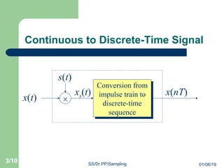
- 3. Continuous to Discrete-Time Signal Conversion from impulse train to discrete-time sequence Conversion from impulse train to discrete-time sequence x(t) x(nT) Ã s(t) xs(t) 01/06/19 3/10 SS/Dr.PP/Sampling
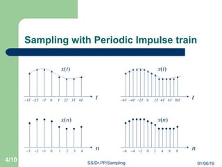
- 4. Sampling with Periodic Impulse train t x(t) 0 T 2T 3T 4TâTâ2Tâ3T n x(n) 0 1 2 3 4â1â2â3 t x(t) 0 2T 4T 8T 10Tâ2Tâ4Tâ8T n x(n) 0 2 4 6 8â2â4â6 01/06/19 4/10 SS/Dr.PP/Sampling
- 5. Sampling with Periodic Impulse train t x(t) 0 T 2T 3T 4TâTâ2Tâ3T n x(n) 0 1 2 3 4â1â2â3 t x(t) 0 2T 4T 8T 10Tâ2Tâ4Tâ8T n x(n) 0 2 4 6 8â2â4â6 What condition has to be placed on the sampling rate? What condition has to be placed on the sampling rate? We want to restore x(t) from x(n).We want to restore x(t) from x(n). 01/06/19 5/10 SS/Dr.PP/Sampling
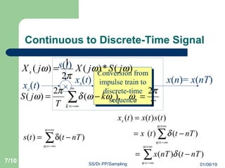
- 6. Continuous to Discrete-Time Signal Conversion from impulse train to discrete-time sequence Conversion from impulse train to discrete-time sequence x (t) x(nT) à s(t) xs(t) â â= ââ= âÎī= n n nTtts )()( )()()( tstxtxs = â â= ââ= â= n n nTttx )()( Îī â â= ââ= â= n n nTtnTx )()( Îī 01/06/19 6/10 SS/Dr.PP/Sampling
- 7. Continuous to Discrete-Time Signal Conversion from impulse train to discrete-time sequence Conversion from impulse train to discrete-time sequence xc(t) x(n)= x(nT) à s(t) xs(t) â â= ââ= âÎī= n n nTtts )()( )()()( tstxtxs = â â= ââ= â= n n nTttx )()( Îī â â= ââ= â= n n nTtnTx )()( Îī )(*)( 2 1 )( ÏÏ Ï Ï jSjXjXs = T k T jS s k s Ï ÏÏÏÎī Ï Ï 2 ,)( 2 )( =â= â â ââ= 01/06/19 7/10 SS/Dr.PP/Sampling
- 8. Continuous to Discrete-Time Signal )(*)( 2 1 )( ÏÏ Ï Ï jSjXjXs = T k T jS s k s Ï ÏÏÏÎī Ï Ï 2 ,)( 2 )( =â= â â ââ= Ïs: Sampling Frequency ïĢ· ïĢļ ïĢķ ïĢŽ ïĢ ïĢŦ â= â â ââ=k ss k T jXjX )( 2 *)( 2 1 )( ÏÏÎī Ï Ï Ï Ï 01/06/19 8/10 SS/Dr.PP/Sampling
- 9. Continuous to Discrete-Time Signal ïĢ· ïĢļ ïĢķ ïĢŽ ïĢ ïĢŦ â= â â ââ=k ss k T jXjX )( 2 *)( 2 1 )( ÏÏÎī Ï Ï Ï Ï â â ââ= â= k skjX T )(*)( 1 ÏÏÎīÏ â â ââ= â= k skjX T ))(( 1 ÏÏ â â ââ= â= k ss kjX T jX ))(( 1 )( ÏÏÏ Therefore Xs(jÏ) is a periodic function of Ï, consisting of a superposition of shifted replicas of X(jÏ), scaled by 1/T. 01/06/19 9/10 SS/Dr.PP/Sampling
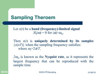
- 10. Sampling Theroem Let x(t) be a band (frequency)-limited signal X(jÏ) = 0 for |Ï|>ÏM. Then x(t) is uniquely determined by its samples {x(nT)} when the sampling frequency satisfies: where Ïs=2Ï/T. 2ÏM is known as the Nyquist rate, as it represents the largest frequency that can be reproduced with the sample time 01/06/1910/10 SS/Dr.PP/Sampling

