�ݺ�ߣ

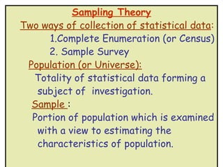
Sampling Theory
Two ways of collection of statistical data:
1.Complete Enumeration (or Census)
2. Sample Survey
Population (or Universe):
Totality of statistical data forming a
subject of investigation.
Sample :
Portion of population which is examined
with a view to estimating the
characteristics of population.

Methods of Sampling

1.Simple Random Sampling
a) [Simple Random Sampling without replacement]
b) [Simple Random Sampling with replacement]

2. Systematic Sampling

3.Stratified Sampling

4.Cluster Sampling

5.Quota Sampling

6. Purposive Sampling ( or Judgment Sampling)

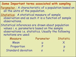
Some Important terms associated with sampling
Parameter : A characteristic of a population based on
all the units of the population.
Statistics: A statistical measure of sample
observation and as such it is a function of sample
observations.
Statistical inferences are drawn about population
values i. e. parameters based on the sample
observations i.e. statistics. Usually the following
notations are used:
Measure Parameter Statistic
Mean μ X
Proportion P p
Standard deviation σ s

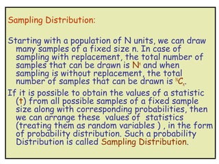
Sampling Distribution:

Starting with a population of N units, we can draw
many samples of a fixed size n. In case of
sampling with replacement, the total number of
samples that can be drawn is Nn and when
sampling is without replacement, the total
number of samples that can be drawn is NCn.
If it is possible to obtain the values of a statistic
(t) from all possible samples of a fixed sample
size along with corresponding probabilities, then
we can arrange these values of statistics
(treating them as random variables ) , in the form
of probability distribution. Such a probability
Distribution is called Sampling Distribution.

Basic Statistical Laws:
1. Law of Statistical Regularity:- It states that a
reasonably large number of items selected at random
from a large group of items, will on the average represent
the characteristics of the group.

2. Law of Inertia of Large Number: It states that large
groups of data show high degree of stability because
there is a greater possibility that one side are
compensated by the extremes on the other side.

3. Central Limit Theorem : If x1, x2, x3, …….. xn is a random
sample of size n drawn from any population (having mean µ
and variance σ2), then the distribution sample mean (x) is
normally distributed with mean µ and variance σ2/n,
provided n is sufficiently large, i.e. n→∞, where µ and σ2
respectively are population mean and variance.

The Mean of the statistic is called ‘Expectation’ and standard
deviation of statistic t is called Standard Error.

Standard Errors (S.E.) of common statistics:

Statistic Standard Error(S.E.)
1.Single Mean (x) : σ/√n
2.Differences of Means (x-y) : √[σ’ 2/n’ + σ”2/n” ]
3. Single Proportion (p) : √[PQ/n]
4. Differences of proportion (p’-p”): √[PQ(1/ n’ +1/ n”]

The factor √[N-n / N-1] is known as finite population
correction factor (fpc)
This is ignored for large population. It is used when n/N is
greater than 0.05

Examples :
1. A simple random sample of size 36 is drawn from
finite population consisting of 101 units. If the
population S.D. is 12.6, find the standard error
of sample mean when the sample is drawn
(a) with replacement (b) without
replacement .
[Ans: a) 2.1 b) 1.69]

2. A random sample of 500 oranges was taken
from a large consignment and 65 were found to
be defective. Show that the S.E. of the
proportion of bad ones in a sample of this size is
0.015.

Theory of Estimation :

Point Estimation ; When a single sample value (t) is used to
estimate parameter (θ), is called point estimation.

Interval Estimation: Instead of estimating parameter θ by a
single value, an interval of values is defined. It specifies two
values that contains unknown parameter.
i.e. P ( t ’≤ θ ≤ t” ) = 1 – α. Then [ t’ , t” ] is called confidence
interval.
α is called level of significance e.g. 5% or 1% l.o.s.
1 – α is called confidence level e.g. 95% or 99% .
Confidence Level
The confidence level is the probability value associated with a
confidence interval.
It is often expressed as a percentage. For example, say , then
the confidence level is equal to (1-0.05) = 0.95, i.e. a 95%
confidence level.

Determination of sample size for Mean :

The following factors must be known:
i) The desired confidence level.
ii) The permissible sampling error E = x - µ.
iii) The standard deviation σ.

The size of sample mean n is given by

n = ( σ Z / E )2 .

Determination of sample size for
Proportion:

The following factors must be known:
i) The desired confidence level.
ii) The permissible sampling error E = P - p.
iii) The estimated true proportion of success.

The size of sample mean n is given by

n = ( Z2pq / E 2 ). Where q = 1-p

Problems:
1. It is known that the population standard deviation in waiting time
for L.P.G. gas cylinder in Delhi is 15 days. How large a sample
should be chosen to be 95% confident, the waiting time is within
7 days of true average. [18]

2. A manufacturing concern wants to estimate the average amount
of purchase of its product in a month by the customers whose
standard error is Rs.10. Find the sample size if the maximum
error is not to exceed Rs.3 with a probability of 0.99 [74]

3. The business manager of a large company wants to check the
inventory records against the physical inventories by a sample
survey. He wants to almost assure that maximum sampling error
should not be more than 5% or below the true proportion of
accurate records. The proportion of accurate records is
estimated as 35% from past experience. Determine the sample
size. [819]
**

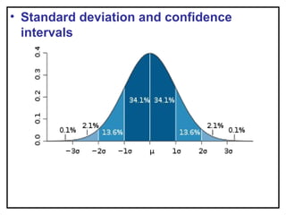
• Standard deviation and confidence
intervals

If t is statistic then

95% confidence interval is given by
[ t ± 1.96 S.E.of t]
99% confidence interval is given by
[ t ± 2.58 S.E.of t]

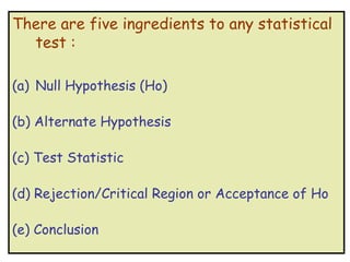
There are five ingredients to any statistical
test :

(a) Null Hypothesis (Ho)

(b) Alternate Hypothesis

(c) Test Statistic

(d) Rejection/Critical Region or Acceptance of Ho

(e) Conclusion

Null Hypothesis
H0: there is no significant difference between the
two values (i. e. statistic and parameter or two
sample values)

Alternative hypothesis
H1: The above difference is significant
[the statement to be accepted if the null is
rejected ]

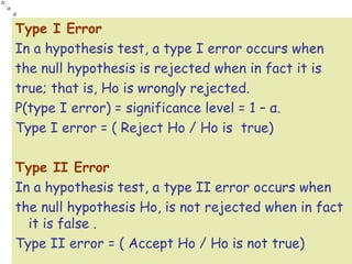
Type I Error
In a hypothesis test, a type I error occurs when
the null hypothesis is rejected when in fact it is
true; that is, Ho is wrongly rejected.
P(type I error) = significance level = 1 – α.
Type I error = ( Reject Ho / Ho is true)

Type II Error
In a hypothesis test, a type II error occurs when
the null hypothesis Ho, is not rejected when in fact
it is false .
Type II error = ( Accept Ho / Ho is not true)

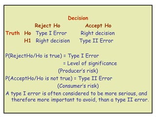
Decision
Reject Ho Accept Ho
Truth Ho Type I Error Right decision
H1 Right decision Type II Error

P(RejectHo/Ho is true) = Type I Error
= Level of significance
(Producer’s risk)
P(AcceptHo/Ho is not true) = Type II Error
(Consumer’s risk)
A type I error is often considered to be more serious, and
therefore more important to avoid, than a type II error.

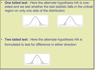
• One tailed test : Here the alternate hypothesis HA is one-
sided and we test whether the test statistic falls in the critical
region on only one side of the distribution

• Two tailed test : Here the alternate hypothesis HA is
formulated to test for difference in either direction

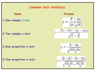
Common test statistics

Name Formula

1.One-sample z-test

2.Two-sample z-test

3.One-proportion z-test

4.Two-proportion z-test,

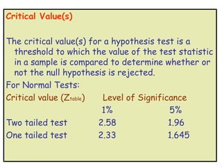
Critical Value(s)

The critical value(s) for a hypothesis test is a
threshold to which the value of the test statistic
in a sample is compared to determine whether or
not the null hypothesis is rejected.
For Normal Tests:
Critical value (Ztable) Level of Significance
1% 5%
Two tailed test 2.58 1.96
One tailed test 2.33 1.645

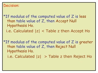
Decision:

*If modulus of the computed value of Z is less
than table value of Z, then Accept Null
Hypothesis Ho.
i.e. Calculated |z| < Table z then Accept Ho

*If modulus of the computed value of Z is greater
than table value of Z, then Reject Null
Hypothesis Ho.
i.e. Calculated |z| > Table z then Reject Ho

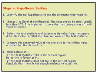
Steps in Hypothesis Testing
1. Identify the null hypothesis Ho and the alternate hypothesis H A.

2. Choose 1- α (level of significance). The value should be small, usually
less than 10%. It is important to consider the consequences of both
types of errors.

3. Select the test statistic and determine its value from the sample
data. This value is called the observed value of the test statistic.

4. Compare the observed value of the statistic to the critical value
obtained for the chosen l.o.s..

5. Make a decision. :
-If the test statistic falls in the critical region:
Reject Ho in favour of H1.
-If the test statistic does not fall in the critical region:
Conclude that there is not enough evidence to reject Ho.

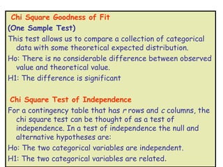
Chi Square Goodness of Fit
(One Sample Test)
This test allows us to compare a collection of categorical
data with some theoretical expected distribution.
Ho: There is no considerable difference between observed
value and theoretical value.
H1: The difference is significant

Chi Square Test of Independence
For a contingency table that has r rows and c columns, the
chi square test can be thought of as a test of
independence. In a test of independence the null and
alternative hypotheses are:
Ho: The two categorical variables are independent.
H1: The two categorical variables are related.

Calculate the chi square statistic x2 by completing
the following steps:
1.For each observed number in the table subtract
the corresponding expected number (O — E).

2.Square the difference [ (O —E)2 ].

3.Divide the squares obtained for each cell in the
table by the expected number for that cell
[ (O - E)2 / E ].

4.Sum all the values for (O - E)2 / E. This is the chi
square statistic .

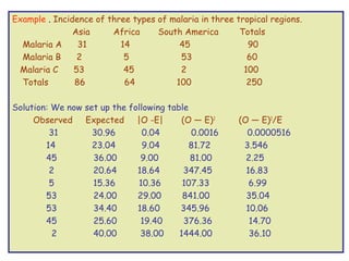
Example . Incidence of three types of malaria in three tropical regions.
Asia Africa South America Totals
Malaria A 31 14 45 90
Malaria B 2 5 53 60
Malaria C 53 45 2 100
Totals 86 64 100 250

Solution: We now set up the following table
Observed Expected |O -E| (O — E) 2 (O — E)2/E
31 30.96 0.04 0.0016 0.0000516
14 23.04 9.04 81.72 3.546
45 36.00 9.00 81.00 2.25
2 20.64 18.64 347.45 16.83
5 15.36 10.36 107.33 6.99
53 24.00 29.00 841.00 35.04
53 34.40 18.60 345.96 10.06
45 25.60 19.40 376.36 14.70
2 40.00 38.00 1444.00 36.10

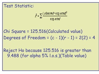
Test Statistic:

Chi Square = 125.516(Calculated value)
Degrees of Freedom = (c - 1)(r - 1) = 2(2) = 4

Reject Ho because 125.516 is greater than
9.488 (for alpha 5% l.o.s.)(Table value)

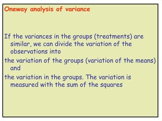
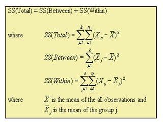
Oneway analysis of variance

If the variances in the groups (treatments) are
similar, we can divide the variation of the
observations into
the variation of the groups (variation of the means)
and
the variation in the groups. The variation is
measured with the sum of the squares

Analysis of Variance (By Coding Method)
Steps in Short Cut Method
1.Set the null hypothesis Ho & Alternate hypothesis H1
2. Steps of computing test statistic
i] Find the sum of all the values of all the items of all the
samples (T)
ii] Compute the correction factor C = square of T / N
N – the total number of observations of all the samples.
iii] Find sum of squares of all the items of all the samples.
iv] Find the total sum of squares SST [ Total in (iii) – C]
v] Find sum of squares between the samples SSC.
[Square the totals of the sample total ,divide by no. of
elements in that samples & subtract C from it.]
vi] Set up ANOVA table and calculate F, which is the test
statistic.
vii] If calculated F is less than table F , Accept Ho otherwise
Reject Ho.

ANOVA Table
Source of Sum of d.o.f. Mean Squares F
variation squares

Between SSC c-1 MSC=SSC/c-1
Samples

Within SSE c(r-1) MSE=SSE/ c(r-1) MSC/MS
Samples [orMSE/MSC]
(As F ratio is
greater than 1)
Total SST cr-1 -

�ݺ�ߣ

Sampling theory

More Related Content

Sampling theory