�ݺ�ߣ

SPEECH COMPRESSION
USING LPC
Prepared By,
Disha Modi,
Roll No: 15MECC12, M.Tech (Communication),
Electronics and Communication Department, NU-IT

Table of Content
• Objective
• Introduction to LPC
• LPC system implementation
• Applications
• Simulation results
• Conclusion

Objective:
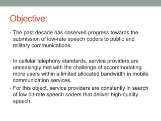
• The past decade has observed progress towards the
submission of low-rate speech coders to public and
military communications.
• In cellular telephony standards, service providers are
unceasingly met with the challenge of accommodating
more users within a limited allocated bandwidth in mobile
communication services.
• For this object, service providers are constantly in search
of low bit-rate speech coders that deliver high-quality
speech.

Introduction to LPC
• Human speech is produced in the vocal tract. The linear
predictive coding (LPC) model is based on the vocal tract
characterized by this tube of a varying diameter and it
represented in mathematical approximation.
• The important facet of LPC is the linear predictive filter
which determines the value of the next sample by a linear
combination of previous samples.
• One important thing about speech production is that
mechanically there is a high correlation between adjacent
samples of speech.
• It is a lossy form of compression.

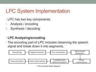
LPC System Implementation
• LPC has two key components:
1. Analysis / encoding
2. Synthesis / decoding
• LPC Analyzing/encoding
• The encoding part of LPC includes observing the speech
signal and break down it into segments.
• LPC encoder block diagram

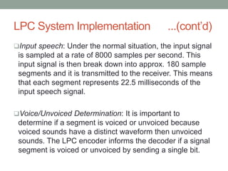
LPC System Implementation ...(cont’d)
Input speech: Under the normal situation, the input signal
is sampled at a rate of 8000 samples per second. This
input signal is then break down into approx. 180 sample
segments and it is transmitted to the receiver. This means
that each segment represents 22.5 milliseconds of the
input speech signal.
Voice/Unvoiced Determination: It is important to
determine if a segment is voiced or unvoiced because
voiced sounds have a distinct waveform then unvoiced
sounds. The LPC encoder informs the decoder if a signal
segment is voiced or unvoiced by sending a single bit.

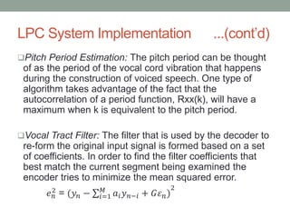
Pitch Period Estimation: The pitch period can be thought
of as the period of the vocal cord vibration that happens
during the construction of voiced speech. One type of
algorithm takes advantage of the fact that the
autocorrelation of a period function, Rxx(k), will have a
maximum when k is equivalent to the pitch period.
Vocal Tract Filter: The filter that is used by the decoder to
re-form the original input signal is formed based on a set
of coefficients. In order to find the filter coefficients that
best match the current segment being examined the
encoder tries to minimize the mean squared error.
𝑒 𝑛
2 = (𝑦𝑛 − 𝑖=1
𝑀
𝑎𝑖 𝑦 𝑛−𝑖 + 𝐺𝜀 𝑛)
2

•
𝑑
𝑑𝑎 𝑗
E[(𝑦𝑛 − 𝑖=1
𝑀
𝑎𝑖 𝑦 𝑛−𝑖 + 𝐺𝜀 𝑛)
2
]=0
• -2E[(𝑦𝑛 − 𝑖=1
𝑀
𝑎𝑖 𝑦 𝑛−𝑖 + 𝐺𝜀 𝑛)𝑦 𝑛−𝑗]=0
• 𝑖=1
𝑀
𝑎𝑖 𝐸 𝑦 𝑛−𝑖 𝑦 𝑛−𝑗 = 𝐸 𝑦 𝑛−𝑖 𝑦 𝑛−𝑗
• In autocorrelation, each E 𝑦 𝑛−𝑖 𝑦 𝑛−𝑗 is converted into an
autocorrelation function of the form Ryy(k) can be
expressed as follows.
• Using Ryy(k), the M equations that were acquired can be
written in matrix form RA = P where A is filter coefficients

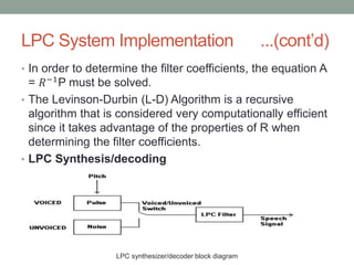
• In order to determine the filter coefficients, the equation A
= 𝑅−1P must be solved.
• The Levinson-Durbin (L-D) Algorithm is a recursive
algorithm that is considered very computationally efficient
since it takes advantage of the properties of R when
determining the filter coefficients.
• LPC Synthesis/decoding
LPC synthesizer/decoder block diagram

• The process of decoding a sequence of speech segments
is the reverse of the encoding process. Each segment is
decoded individually.
• Each segment of speech has a different LPC filter that is
eventually produced using the reflection coefficients and
the gain that are received from the encoder.
• The final step of decoding a segment of speech is to pass
the excitement signal through the filter to produce the
synthesized speech signal.

Applications
• Standard telephone systems
• Voice mail systems
• Telephone auto answering machines
• Text to speech synthesis
• Multimedia
• Used in the tonal analysis of violins and other stringed
musical instruments
• SILK audio codec
• other lossless audio codecs

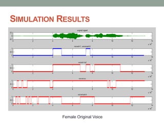
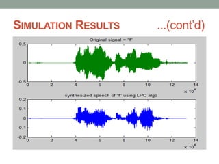
SIMULATION RESULTS
Female Original Voice

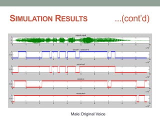
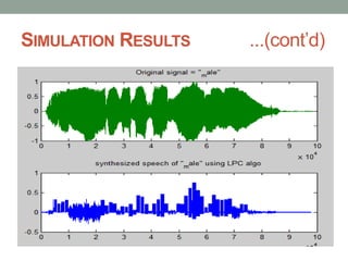
SIMULATION RESULTS ...(cont’d)

Male Original Voice

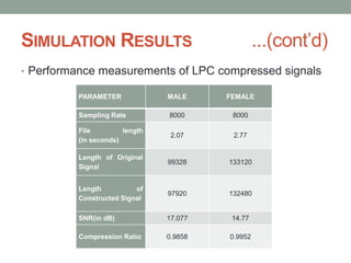
• Performance measurements of LPC compressed signals
PARAMETER MALE FEMALE
Sampling Rate 8000 8000
File length
(in seconds)
2.07 2.77
Length of Original
Signal
99328 133120
Length of
Constructed Signal
97920 132480
SNR(in dB) 17.077 14.77
Compression Ratio 0.9858 0.9952

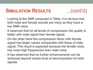
• Looking at the SNR computed in Table, it is obvious that
both male and female sounds are noisy as they have a
low SNR value.
• It observed that for all levels of compression the quality is
better with male signal than female signal.
• On the other hand the compression factor with female
signal has larger values comparable with these of male
signal. This result is expected because the female voice
has more high frequencies than male voice.
• It has observed that no further enhancements can be
achieved beyond certain level of decomposition for both
signals.

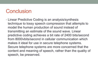
Conclusion
• Linear Predictive Coding is an analysis/synthesis
technique to lossy speech compression that attempts to
model the human production of sound instead of
transmitting an estimate of the sound wave. Linear
predictive coding achieves a bit rate of 2400 bits/second
from 8000vbits/second in cellular communication which
makes it ideal for use in secure telephone systems.
Secure telephone systems are more concerned that the
content and meaning of speech, rather than the quality of
speech, be preserved.

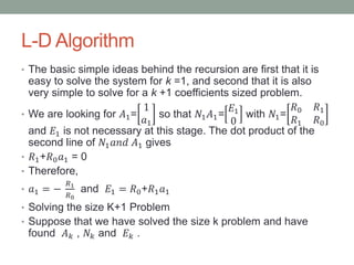
L-D Algorithm
• The basic simple ideas behind the recursion are first that it is
easy to solve the system for k =1, and second that it is also
very simple to solve for a k +1 coefficients sized problem.
• We are looking for 𝐴1=
1
𝑎1
so that 𝑁1 𝐴1=
𝐸1
0
with 𝑁1=
𝑅0 𝑅1
𝑅1 𝑅0
and 𝐸1 is not necessary at this stage. The dot product of the
second line of 𝑁1 𝑎𝑛𝑑 𝐴1 gives
• 𝑅1+𝑅0 𝑎1 = 0
• Therefore,
• 𝑎1 = −
𝑅1
𝑅0
and 𝐸1 = 𝑅0+𝑅1 𝑎1
• Solving the size K+1 Problem
• Suppose that we have solved the size k problem and have
found 𝐴 𝑘 , 𝑁𝑘 and 𝐸 𝑘 .

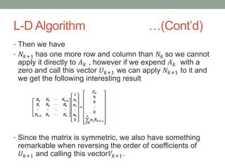
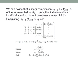
L-D Algorithm …(Cont’d)
• Then we have
• 𝑁𝑘+1 has one more row and column than 𝑁𝑘 so we cannot
apply it directly to 𝐴 𝑘 , however if we expend 𝐴 𝑘 with a
zero and call this vector 𝑈 𝑘+1 we can apply 𝑁𝑘+1 to it and
we get the following interesting result
• Since the matrix is symmetric, we also have something
remarkable when reversing the order of coefficients of
𝑈 𝑘+1 and calling this vector𝑉𝑘+1.

• We can notice that a linear combination 𝑈 𝑘+1 + 𝜆 𝑉𝑘+1 is
of the form wanted for 𝐴 𝑘+1 since the first element is a 1
for all values of 𝜆 . Now if there was a value of 𝜆 for
• Calculating 𝑁𝑘+1 (𝑈 𝑘+1+𝜆) gives

�ݺ�ߣ

Speech Compression using LPC

More Related Content

Speech Compression using LPC