


![SVM[Support vector Machine] Machine learning](https://cdn.slidesharecdn.com/ss_thumbnails/svm-250403184638-1cd9afdb-thumbnail.jpg?width=560&fit=bounds)


More Related Content
Similar to Statistical Machine Learning unit4 lecture notes (20)
More from SureshK256753 (7)


Recently uploaded (20)


Statistical Machine Learning unit4 lecture notes
- 1. UNIT-4 SML
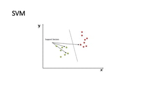
- 2. SVM ŌĆó Support Vector MachineŌĆØ (SVM) is a supervised machine learning algorithm that can be used for both classification or regression challenges. ŌĆó However, it is mostly used in classification problems. ŌĆó In the SVM algorithm, we plot each data item as a point in n-dimensional space (where n is a number of features you have) with the value of each feature being the value of a particular coordinate. ŌĆó Then, we perform classification by finding the hyper-plane that differentiates the two classes very well.
- 3. SVM ŌĆó Imagined as a surface that maximizes the boundaries between various types of points of data that is represent in multidimensional space, also known as a hyperplane, which creates the most homogeneous points in each subregion. ŌĆó Support vector machines can be used on any type of data, but have special extra advantages for data types with very high dimensions relative to the observations, for example Text classification, in which language has the very dimensions of word vectors For the quality control of DNA sequencing by labeling chromatograms correctly
- 4. Support vector machines working principles ŌĆó Support vector machines are mainly classified into three types based on their ŌĆó working principles: - Maximum margin classifiers - - Support vector classifiers - Support vector machines
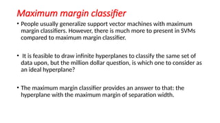
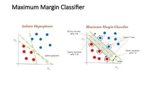
- 5. Maximum margin classifier ŌĆó People usually generalize support vector machines with maximum margin classifiers. However, there is much more to present in SVMs compared to maximum margin classifier. ŌĆó It is feasible to draw infinite hyperplanes to classify the same set of data upon, but the million dollar question, is which one to consider as an ideal hyperplane? ŌĆó The maximum margin classifier provides an answer to that: the hyperplane with the maximum margin of separation width.
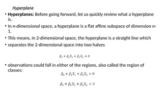
- 6. Hyperplane ŌĆó Hyperplanes: Before going forward, let us quickly review what a hyperplane is. ŌĆó In n-dimensional space, a hyperplane is a flat affine subspace of dimension n- 1. ŌĆó This means, in 2-dimensional space, the hyperplane is a straight line which ŌĆó separates the 2-dimensional space into two halves ŌĆó observations could fall in either of the regions, also called the region of classes:
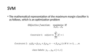
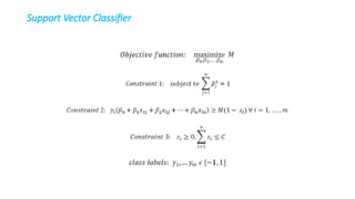
- 7. SVM ŌĆó The mathematical representation of the maximum margin classifier is as follows, which is an optimization problem
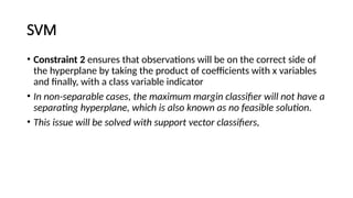
- 8. SVM ŌĆó Constraint 2 ensures that observations will be on the correct side of the hyperplane by taking the product of coefficients with x variables and finally, with a class variable indicator ŌĆó In non-separable cases, the maximum margin classifier will not have a separating hyperplane, which is also known as no feasible solution. ŌĆó This issue will be solved with support vector classifiers,
- 10. SVM
- 11. How does it work? ŌĆó the process of segregating the two classes with a hyper-plane. ŌĆó How can we identify the right hyper-plane?
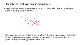
- 12. Identify the right hyper-plane (Scenario-1): ŌĆó Here, we have three hyper-planes (A, B, and C). Now, identify the right hyper- plane to classify stars and circles. ŌĆó You need to remember a thumb rule to identify the right hyper-plane: ŌĆ£Select the hyper-plane which segregates the two classes betterŌĆØ. In this scenario, hyper- plane ŌĆ£BŌĆØ has excellently performed this job
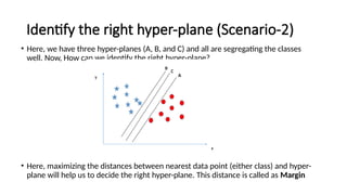
- 13. Identify the right hyper-plane (Scenario-2) ŌĆó Here, we have three hyper-planes (A, B, and C) and all are segregating the classes well. Now, How can we identify the right hyper-plane? ŌĆó Here, maximizing the distances between nearest data point (either class) and hyper- plane will help us to decide the right hyper-plane. This distance is called as Margin
- 14. you can see that the margin for hyper-plane C is high as compared to both A and B. Hence, we name the right hyper- plane as C. Another lightning reason for selecting the hyper- plane with higher margin is robustness. If we select a hyper- plane having low margin then there is high chance of miss- classification.
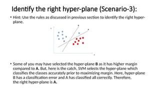
- 15. Identify the right hyper-plane (Scenario-3): ŌĆó Hint: Use the rules as discussed in previous section to identify the right hyper- plane. ŌĆó Some of you may have selected the hyper-plane B as it has higher margin compared to A. But, here is the catch, SVM selects the hyper-plane which classifies the classes accurately prior to maximizing margin. Here, hyper-plane B has a classification error and A has classified all correctly. Therefore, the right hyper-plane is A.
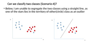
- 16. Can we classify two classes (Scenario-4)? ŌĆó Below, I am unable to segregate the two classes using a straight line, as one of the stars lies in the territory of other(circle) class as an outlier
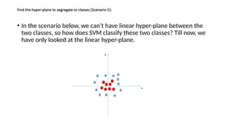
- 17. Find the hyper-plane to segregate to classes (Scenario-5): ŌĆó In the scenario below, we canŌĆÖt have linear hyper-plane between the two classes, so how does SVM classify these two classes? Till now, we have only looked at the linear hyper-plane.
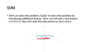
- 18. SVM ŌĆó SVM can solve this problem. Easily! It solves this problem by introducing additional feature. Here, we will add a new feature z=x^2+y^2. Now, letŌĆÖs plot the data points on axis x and z:
- 19. Support vector classifier ŌĆó Support vector classifiers are an extended version of maximum margin classifiers, in which some violations are tolerated for non-separable cases in order to create the best fit, even with slight errors within the threshold limit. ŌĆó In fact, in real-life scenarios, we hardly find any data with purely separable classes; most classes have a few or more observations in overlapping classes. ŌĆó The mathematical representation of the support vector classifier is as follows, a slight correction to the constraints to accommodate error terms.
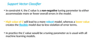
- 21. Support Vector Classifier ŌĆó In constraint 4, the C value is a non-negative tuning parameter to either accommodate more or fewer overall errors in the model. ŌĆó High value of C will lead to a more robust model, whereas a lower value creates the flexible model due to less violation of error terms. ŌĆó In practice the C value would be a tuning parameter as is usual with all machine learning models.
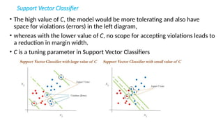
- 22. Support Vector Classifier ŌĆó The high value of C, the model would be more tolerating and also have space for violations (errors) in the left diagram, ŌĆó whereas with the lower value of C, no scope for accepting violations leads to a reduction in margin width. ŌĆó C is a tuning parameter in Support Vector Classifiers
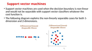
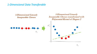
- 23. Support vector machines ŌĆó Support vector machines are used when the decision boundary is non-linear and would not be separable with support vector classifiers whatever the cost function is. ŌĆó The following diagram explains the non-linearly separable cases for both 1- dimension and 2-dimensions.
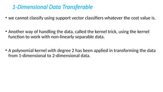
- 24. 1-Dimensional Data Transferable ŌĆó we cannot classify using support vector classifiers whatever the cost value is. ŌĆó Another way of handling the data, called the kernel trick, using the kernel function to work with non-linearly separable data. ŌĆó A polynomial kernel with degree 2 has been applied in transforming the data from 1-dimensional to 2-dimensional data.
- 26. 1-Dimensional Data Transferable ŌĆó The degree of the polynomial kernel is a tuning parameter ŌĆó The practitioner needs to tune them with various values to check where higher accuracies are possible with the model
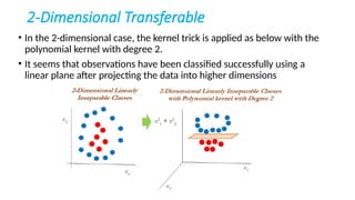
- 27. 2-Dimensional Transferable ŌĆó In the 2-dimensional case, the kernel trick is applied as below with the polynomial kernel with degree 2. ŌĆó It seems that observations have been classified successfully using a linear plane after projecting the data into higher dimensions
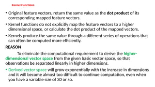
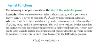
- 28. Kernel Functions ŌĆó Original feature vectors, return the same value as the dot product of its corresponding mapped feature vectors. ŌĆó Kernel functions do not explicitly map the feature vectors to a higher dimensional space, or calculate the dot product of the mapped vectors. ŌĆó Kernels produce the same value through a different series of operations that can often be computed more efficiently. REASON To eliminate the computational requirement to derive the higher- dimensional vector space from the given basic vector space, so that observations be separated linearly in higher dimensions. ŌĆó Derived vector space will grow exponentially with the increase in dimensions and it will become almost too difficult to continue computation, even when you have a variable size of 30 or so.
- 29. Kernel Functions ŌĆó The following example shows how the size of the variables grows.
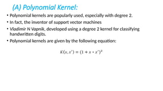
- 30. (A) Polynomial Kernel: ŌĆó Polynomial kernels are popularly used, especially with degree 2. ŌĆó In fact, the inventor of support vector machines ŌĆó Vladimir N Vapnik, developed using a degree 2 kernel for classifying handwritten digits. ŌĆó Polynomial kernels are given by the following equation:
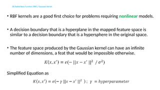
- 31. (B) Radial Basis Function (RBF) / Gaussian Kernel: ŌĆó RBF kernels are a good first choice for problems requiring nonlinear models. ŌĆó A decision boundary that is a hyperplane in the mapped feature space is similar to a decision boundary that is a hypersphere in the original space. ŌĆó The feature space produced by the Gaussian kernel can have an infinite number of dimensions, a feat that would be impossible otherwise. Simplified Equation as
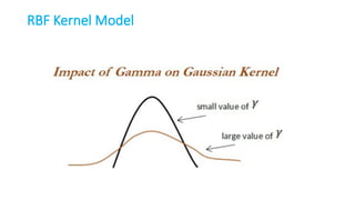
- 32. RBF Kernel Model
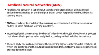
- 33. Artificial Neural Networks (ANN) ŌĆó Relationship between a set of input signals and output signals using a model derived from a replica of the biological brain, which responds to stimuli from its sensory inputs. ŌĆó ANN methods try to model problems using interconnected artificial neurons (or nodes) to solve machine learning problems. ŌĆó Incoming signals are received by the cell's dendrites through a biochemical process that allows the impulses to be weighted according to their relative importance. ŌĆó The cell body begins to accumulate the incoming signals, a threshold is reached, at which the cell fires and the output signal is then transmitted via an electrochemical process down the axon
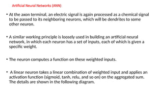
- 34. Artificial Neural Networks (ANN) ŌĆó At the axon terminal, an electric signal is again processed as a chemical signal to be passed to its neighboring neurons, which will be dendrites to some other neuron. ŌĆó A similar working principle is loosely used in building an artificial neural network, in which each neuron has a set of inputs, each of which is given a specific weight. ŌĆó The neuron computes a function on these weighted inputs. ŌĆó A linear neuron takes a linear combination of weighted input and applies an activation function (sigmoid, tanh, relu, and so on) on the aggregated sum. The details are shown in the following diagram.
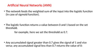
- 35. Artificial Neural Networks (ANN) ŌĆó The network feeds the weighted sum of the input into the logistic function (in case of sigmoid function). ŌĆó The logistic function returns a value between 0 and 1 based on the set threshold. for example, here we set the threshold as 0.7. ŌĆó Any accumulated signal greater than 0.7 gives the signal of 1 and vice versa; any accumulated signal less than 0.7 returns the value of 0:
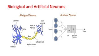
- 36. Biological and Artificial Neurons
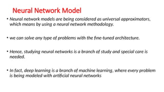
- 37. Neural Network Model ŌĆó Neural network models are being considered as universal approximators, which means by using a neural network methodology. ŌĆó we can solve any type of problems with the fine-tuned architecture. ŌĆó Hence, studying neural networks is a branch of study and special care is needed. ŌĆó In fact, deep learning is a branch of machine learning, where every problem is being modeled with artificial neural networks
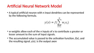
- 38. Artificial Neural Network Model ŌĆó A typical artificial neuron with n input dendrites can be represented by the following formula. ŌĆó w weights allow each of the n inputs of x to contribute a greater or lesser amount to the sum of input signals. ŌĆó The accumulated value is passed to the activation function, f(x), and the resulting signal, y(x), is the output axon
- 39. Parameters- Building neural networks ŌĆó Activation function: Choosing an activation function plays a major role in aggregating signals into the output signal to be propagated to the other neurons of the network. ŌĆó Network architecture or topology: This represents the number of layers required and the number of neurons in each layer. More layers and neurons will create a highly non-linear decision boundary, whereas if we reduce the architecture, the model will be less flexible and more robust. ŌĆó Training optimization algorithm: The selection of an optimization algorithm plays a critical role as well, in order to converge quickly and accurately to the best optimal solutions
- 40. Parameters- Building neural networks ŌĆó Applications of Neural Networks: In recent years, neural networks (a branch of deep learning) has gained huge attention in terms of its application in artificial intelligence, in terms of speech, text, vision, and many other areas. ŌĆó Images and videos: To identify an object in an image or to classify whether it is a dog or a cat ŌĆó Text processing (NLP): Deep-learning-based chatbot and so on ŌĆó Speech: Recognize speech ŌĆó Structured data processing: Building highly powerful models to obtain a non-linear decision boundary
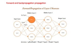
- 41. Forward and backpropagation propagation
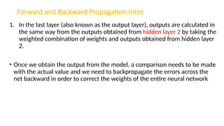
- 42. Forward and Backward Propogation-Intro ŌĆó Forward propagation and backpropagation are illustrated with the two hidden layer deep neural networks in the following example, in which both layers get three neurons each, in addition to input and output layers. ŌĆó The number of neurons in the input layer is based on the number of x (independent) variables, whereas the number of neurons in the output layer is decided by the number of classes the model needs to be predicted. ŌĆó Only one neuron in each layer; however, the reader can attempt to create other neurons within the same layer. Weights and biases are initiated from some random numbers, so that in both forward and backward passes, these can be updated in order to minimize the errors altogether.
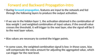
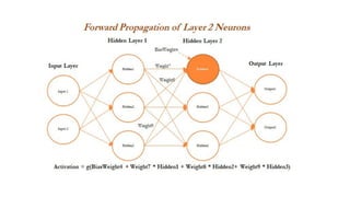
- 43. Forward and Backward Propagation-Intro ŌĆó During forward propagation, features are input to the network and fed through the following layers to produce the output activation. ŌĆó If we see in the hidden layer 1, the activation obtained is the combination of bias weight 1 and weighted combination of input values; if the overall value crosses the threshold, it will trigger to the next layer, else the signal will be 0 to the next layer values. ŌĆó Bias values are necessary to control the trigger points. ŌĆó In some cases, the weighted combination signal is low; in those cases, bias will compensate the extra amount for adjusting the aggregated value, which can trigger for the next level.
- 44. Forward and Backward Propagation-Intro
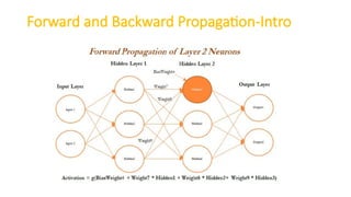
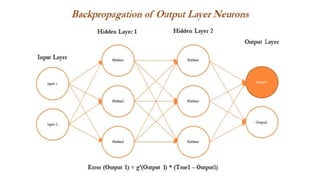
- 45. Forward and Backward Propagation-Intro 1. In the last layer (also known as the output layer), outputs are calculated in the same way from the outputs obtained from hidden layer 2 by taking the weighted combination of weights and outputs obtained from hidden layer 2. ŌĆó Once we obtain the output from the model, a comparison needs to be made with the actual value and we need to backpropagate the errors across the net backward in order to correct the weights of the entire neural network
- 48. Forward and Backward Propagation ŌĆó we have taken the derivative of the output value and multiplied by that much amount to the error component, which was obtained from differencing the actual value with the model output
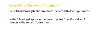
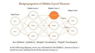
- 50. Forward and Backward Propagation ŌĆó we will backpropagate the error from the second hidden layer as well. ŌĆó In the following diagram, errors are computed from the Hidden 4 neuron in the second hidden layer
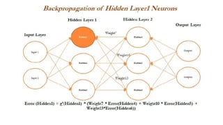
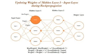
- 53. Forward and Backward Propagation ŌĆó Once all the neurons in hidden layer 1 are updated, weights between inputs and the hidden layer also need to be updated, as we cannot update anything on input variables. ŌĆó we will be updating the weights of both the inputs and also, at the same time, the neurons in hidden layer 1, as neurons in layer 1 utilize the weights from input only
- 56. Forward and Backward Propagation ŌĆó We have not shown the next iteration, in which neurons in the output layer are updated with errors and backpropagation started again. ŌĆó In a similar way, all the weights get updated until a solution converges or the number of iterations is reached.
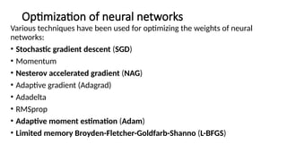
- 57. Optimization of neural networks Various techniques have been used for optimizing the weights of neural networks: ŌĆó Stochastic gradient descent (SGD) ŌĆó Momentum ŌĆó Nesterov accelerated gradient (NAG) ŌĆó Adaptive gradient (Adagrad) ŌĆó Adadelta ŌĆó RMSprop ŌĆó Adaptive moment estimation (Adam) ŌĆó Limited memory Broyden-Fletcher-Goldfarb-Shanno (L-BFGS)
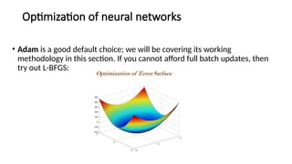
- 58. Optimization of neural networks ŌĆó Adam is a good default choice; we will be covering its working methodology in this section. If you cannot afford full batch updates, then try out L-BFGS:
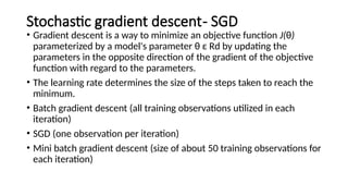
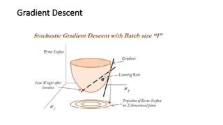
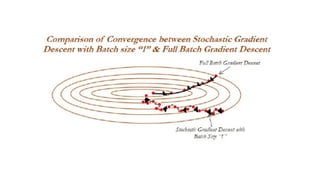
- 59. Stochastic gradient descent- SGD ŌĆó Gradient descent is a way to minimize an objective function J(╬Ė) parameterized by a model's parameter ╬Ė ╬Ą Rd by updating the parameters in the opposite direction of the gradient of the objective function with regard to the parameters. ŌĆó The learning rate determines the size of the steps taken to reach the minimum. ŌĆó Batch gradient descent (all training observations utilized in each iteration) ŌĆó SGD (one observation per iteration) ŌĆó Mini batch gradient descent (size of about 50 training observations for each iteration)
- 60. Gradient Descent