�ݺ�ߣ

Estimation of Retail Demand Under Partially-Observed Out-of-Stocks

Agenda Motivation Big Picture Contribution Model & Methodology Empirical Results Managerial Implications Extensions Conclusions

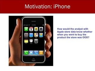
Motivation: iPhone How would the analyst with Apple store data know whether when you went to buy the product the store was OOS?

Big Picture: Many situations in which we don’t observe individual behavior, but we may have some aggregate or limited information. Key: use aggregate data to formulate constraints on the unobserved individual behavior. Dependent variables: Choices Independent variables: Coupon promotions Environment: Out-of-stocks Other applications: Shopping paths

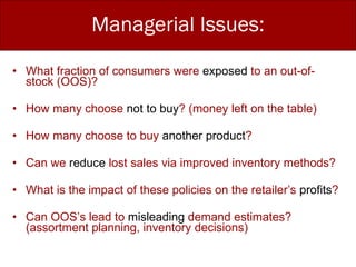
What fraction of consumers were exposed to an out-of-stock (OOS)? How many choose not to buy ? (money left on the table) How many choose to buy another product ? Can we reduce lost sales via improved inventory methods? What is the impact of these policies on the retailer’s profits ? Can OOS’s lead to misleading demand estimates? (assortment planning, inventory decisions) Managerial Issues:

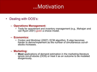
…Motivation Dealing with OOS’s: Operations Management: Tools for assortment and inventory management (e.g., Mahajan and van Ryzin 2001) given a choice model. Economics: Conlon and Mortimer (2007): ECM algorithm, E-step becomes harder to derive/implement as the number of simultaneous out-of-stocks increases. Marketing: Most applications of demand estimation in the marketing literature ignore out-of-stocks (OOS) or treat it as an outcome to be modeled exogenously.

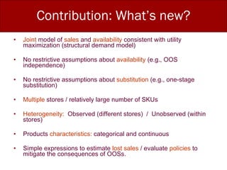
Contribution: What’s new? Joint model of sales and availability consistent with utility maximization (structural demand model) No restrictive assumptions about availability (e.g., OOS independence) No restrictive assumptions about substitution (e.g., one-stage substitution) Multiple stores / relatively large number of SKUs Heterogeneity: Observed (different stores) / Unobserved (within stores) Products characteristics: categorical and continuous Simple expressions to estimate lost sales / evaluate policies to mitigate the consequences of OOSs.

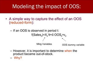
Modeling the impact of OOS: A simple way to capture the effect of an OOS ( reduced-form ): If an OOS is observed in period t: f(Sales jt )=X jt ’  +  OOS jt +  jt However, it is important to determine when the product became out-of-stock. Why? Mktg Variables OOS dummy variable

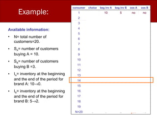
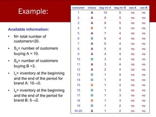
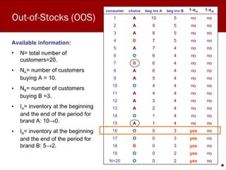
Available information: N= total number of customers=20. S A = number of customers buying A = 10. S B = number of customers buying B =3. I A = inventory at the beginning and the end of the period for brand A: 10  0. I B = inventory at the beginning and the end of the period for brand B: 5  2. Example: no yes 2 0 O N=20 no yes 2 0 O 19 no yes 3 0 B 18 no yes 3 0 O 17 no yes 3 0 O 16 no yes 4 0 B 15 no yes 4 0 O 14 no no 4 1 A 13 no no 4 2 A 12 no no 4 3 A 11 no no 4 3 O 10 no no 4 4 A 9 no no 4 5 A 8 no no 4 6 A 7 no no 4 6 O 6 no no 4 7 A 5 no no 5 7 B 4 no no 5 8 A 3 no no 5 9 A 2 no no 5 10 A 1 oos B oos A beg inv B beg inv A choice consumer

Example: Available information: N= total number of customers=20. S A = number of customers buying A = 10. S B = number of customers buying B =3. I A = inventory at the beginning and the end of the period for brand A: 10  0. I B = inventory at the beginning and the end of the period for brand B: 5  2. no no 2 1 A N=20 no no 2 1 O 19 no no 3 1 B 18 no no 3 1 O 17 no no 3 1 O 16 no no 4 1 B 15 no no 4 1 O 14 no no 4 1 O 13 no no 4 2 A 12 no no 4 3 A 11 no no 4 3 O 10 no no 4 4 A 9 no no 4 5 A 8 no no 4 6 A 7 no no 4 6 O 6 no no 4 7 A 5 no no 5 7 B 4 no no 5 8 A 3 no no 5 9 A 2 no no 5 10 A 1 oos B oos A beg inv B beg inv A choice consumer

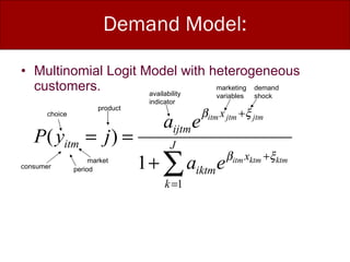
Demand Model: Multinomial Logit Model with heterogeneous customers. consumer product period choice availability indicator marketing variables market demand shock

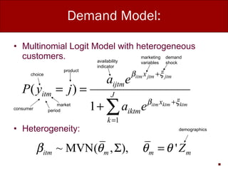
Demand Model: Multinomial Logit Model with heterogeneous customers. Heterogeneity: demographics consumer product period choice availability indicator marketing variables market demand shock

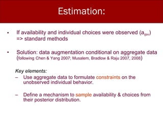
Estimation: If availability and individual choices were observed (a ijtm ) => standard methods Solution: data augmentation conditional on aggregate data ( following Chen & Yang 2007; Musalem, Bradlow & Raju 2007, 2008 ) Key elements: Use aggregate data to formulate constraints on the unobserved individual behavior. Define a mechanism to sample availability & choices from their posterior distribution.

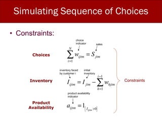
Simulating Sequence of Choices Constraints: choice indicator Choices Inventory Product Availability initial inventory sales inventory faced by customer i product availability indicator Constraints

Available information: N= total number of customers=20. N A = number of customers buying A = 10. N B = number of customers buying B =3. I A = inventory at the beginning and the end of the period for brand A: 10  0. I B = inventory at the beginning and the end of the period for brand B: 5  2. Out-of-Stocks (OOS) no yes 2 0 O N=20 no yes 2 0 O 19 no yes 3 0 B 18 no yes 3 0 O 17 no yes 3 0 O 16 no yes 4 0 B 15 no yes 4 0 O 14 no no 4 1 A 13 no no 4 2 A 12 no no 4 3 A 11 no no 4 3 O 10 no no 4 4 A 9 no no 4 5 A 8 no no 4 6 A 7 no no 4 6 O 6 no no 4 7 A 5 no no 5 7 B 4 no no 5 8 A 3 no no 5 9 A 2 no no 5 10 A 1 1-a iB 1-a iA beg inv B beg inv A choice consumer

Out-of-Stocks (OOS) Available information: N= total number of customers=20. N A = number of customers buying A = 10. N B = number of customers buying B =3. I A = inventory at the beginning and the end of the period for brand A: 10  0. I B = inventory at the beginning and the end of the period for brand B: 5  2. no yes 2 0 O N=20 no yes 2 0 O 19 no yes 3 0 B 18 no yes 3 0 O 17 no yes 3 0 O 16 no no 4 1 A 15 no no 4 1 O 14 no no 4 2 A 13 no no 4 3 A 12 no no 4 4 A 11 no no 4 4 O 10 no no 4 5 A 9 no no 4 6 A 8 no no 4 6 B 7 no no 4 6 O 6 no no 4 7 A 5 no no 5 7 B 4 no no 5 8 A 3 no no 5 9 A 2 no no 5 10 A 1 1-a iB 1-a iA beg inv B beg inv A choice consumer

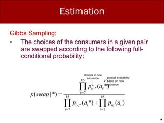
Estimation Gibbs Sampling: The choices of the consumers in a given pair are swapped according to the following full-conditional probability: choices in new sequence product availability based on new sequence

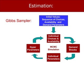
Estimation: Initial Values: Sequence of Choices, Availability and Demand Parameters Individual Choices & Availability Individual Parameters Hyper Parameters Gibbs Sampler: MCMC Simulation Demand Shocks

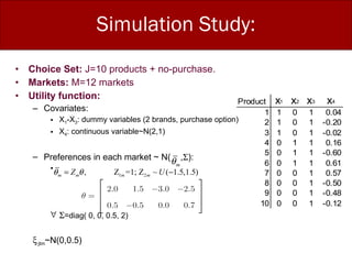
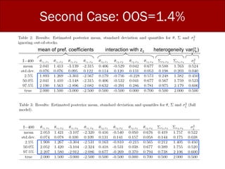
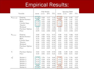
Simulation Study: Choice Set: J=10 products + no-purchase. Markets: M=12 markets Utility function: Covariates: X 1 -X 3 : dummy variables (2 brands, purchase option) X 4 : continuous variable~N(2,1) Preferences in each market ~ N( ,  ):  =diag( 0, 0, 0.5, 2)  jtm ~N(0,0.5)

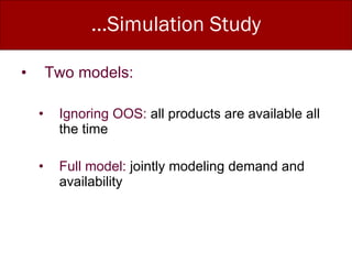
…Simulation Study Two models: Ignoring OOS: all products are available all the time Full model: jointly modeling demand and availability

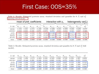
First Case: OOS=35% mean of pref. coefficients interaction with z 2 heterogeneity var(  )

Second Case: OOS=1.4% mean of pref. coefficients interaction with z 2 heterogeneity var(  )

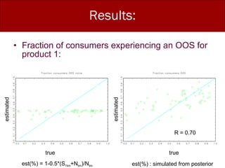
Results: Fraction of consumers experiencing an OOS for product 1: true true estimated estimated est(%) = 1-0.5*(S 1tm +N tm )/N tm est(%) : simulated from posterior R = 0.70

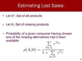
Estimating Lost Sales: Let A*: Set of all products Let A i : Set of missing products Probability of a given consumer having chosen one of the missing alternatives had it been available:

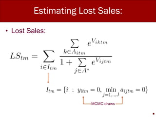
Estimating Lost Sales: Lost Sales: MCMC draws

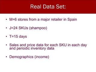
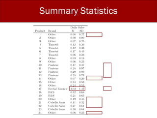
Real Data Set: M=6 stores from a major retailer in Spain J=24 SKUs (shampoo) T=15 days Sales and price data for each SKU in each day and periodic inventory data Demographics (income)

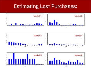
Estimating Lost Purchases: Market 1 Market 2 Market 3 Market 4 Market 5 Market 6

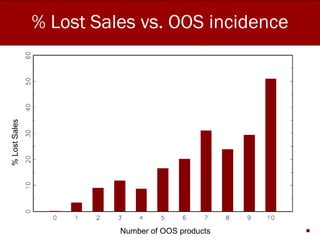
% Lost Sales vs. OOS incidence Number of OOS products % Lost Sales

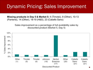
Dynamic Pricing: Sales Improvement Missing products in Day 5 & Market 5: 4 (Timotei), 9 (Other), 10-13 (Pantene), 14 (Other), 18-19 (H&S), 23 (Cabello Sano)

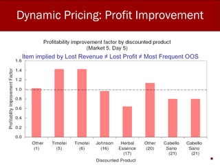
Dynamic Pricing: Profit Improvement Item implied by Lost Revenue ≠ Lost Profit ≠ Most Frequent OOS

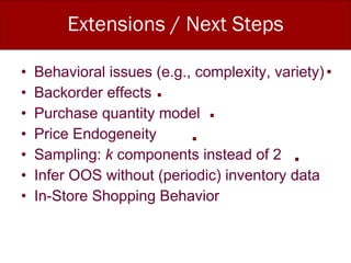
Extensions / Next Steps Behavioral issues (e.g., complexity, variety) Backorder effects Purchase quantity model Price Endogeneity Sampling: k components instead of 2 Infer OOS without (periodic) inventory data In-Store Shopping Behavior

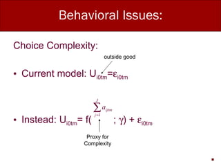
Behavioral Issues: Choice Complexity: Current model: U i0tm =  i0tm Instead: U i0tm = f( ;  ) +  i0tm Proxy for Complexity outside good

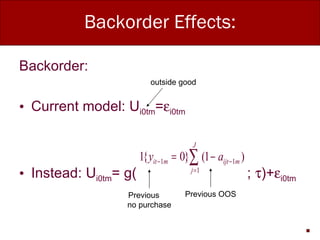
Backorder Effects: Backorder: Current model: U i0tm =  i0tm Instead: U i0tm = g( ;  )+  i0tm Previous OOS outside good Previous no purchase

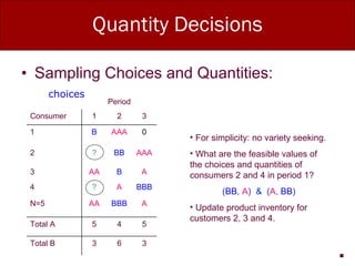
Quantity Decisions Sampling Choices and Quantities: choices For simplicity: no variety seeking. What are the feasible values of the choices and quantities of consumers 2 and 4 in period 1? ( BB , A ) & ( A , BB ) Update product inventory for customers 2, 3 and 4. 5 4 5 Total A BBB A ? 4 AAA BB ? 2 A B AA 3 A BBB AA N=5 3 6 3 Total B 0 AAA B 1 3 2 1 Consumer Period

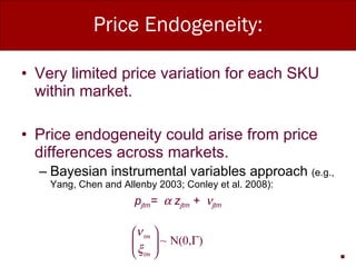
Price Endogeneity: Very limited price variation for each SKU within market. Price endogeneity could arise from price differences across markets. Bayesian instrumental variables approach (e.g., Yang, Chen and Allenby 2003; Conley et al. 2008): p jtm =  z jtm +  jtm

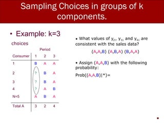
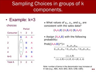
Sampling Choices in groups of k components. Example: k=3 choices What values of y 21 , y 31 and y 41 are consistent with the sales data? ( A , A , B ) ( A , B , A ) ( B , A , A ) Assign ( A , A , B ) with the following probability: Prob(( A , A , B )|*)= B A ? 4 A B ? 2 A B ? 3 A B A N=5 4 2 3 Total A A A B 1 3 2 1 Consumer Period

Sampling Choices in groups of k components. Example: k=3 Note: number of terms in the denominator may increase at k! rate (e.g., ABC, ACA, BAC, BCA, CAB, CBA). choices What values of y 21 , y 31 and y 41 are consistent with the sales data? ( A , A , B ) ( A , B , A ) ( B , A , A ) Assign ( A , A , B ) with the following probability: Prob(( A , A , B )|*)= B A ? 4 A B ? 2 A B ? 3 A B A N=5 4 2 3 Total A A A B 1 3 2 1 Consumer Period

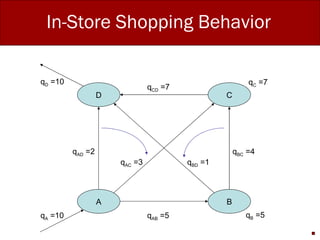
In-Store Shopping Behavior Using RFID technology it is possible to track the location of shopping carts in a grocery store every 5 seconds ( disaggregate data). Alternatively: record the number of shopping carts that pass through a measuring point ( aggregate data). Infer the trajectory of shopping carts using only these aggregate measurements.

In-Store Shopping Behavior A B C D q A =10 q B =5 q C =7 q D =10 q AB =5 q BC =4 q BD =1 q AC =3 q AD =2 q CD =7

Conclusions: Bayesian methods / data augmentation enable us to jointly model choices and product availability w/o restrictive assumptions on: Joint probability of out-of-stocks / substitution Key: use available information to formulate constraints on unobserved individual data: Constraints and Data Augmentation As a byproduct, we obtain simple expressions to: Estimate the magnitude of lost sales Assess effectiveness of policies aimed at mitigating the costs of OOSs Several extensions are possible…

�ݺ�ߣ

Stockout

More Related Content

Stockout

Editor's Notes