Summary distributed representations_words_phrases
- 1. A Summary for Distributed Representations of Words and Phrases and Their Compositionality Xiangnan YUE xiangnanyue@gmail.com Ing¨¦nieur Civil @Mines ParisTech M2 Data Science @Ecole Polytechnique
- 2. Road Map - Part 1 - Learning Word2Vec - Baseline Skip-gram model - Hierarchical softmax - Negative sampling - Sub-sampling trick - Part 2 - Learning Phrase - Part 3 - Empirical Results - Part 4 - Additive Compositionality - Part 5 - Conclusion
- 3. Background This paper follows the paper [1] Efficient estimation of word representations in vector space in 2013. This paper proposed some important improvements for the Skip-gram model, which is widely used for obtaining the famous ˇ°word vectorsˇ±. [1] proposed the CBOW (Continuous Bag-of-words Model) and Skip-gram, using a 3-layer neural network to train the word-vectors. While CBOW is entering the context to predict the center, Skip-gram is entering the center word to predict the context.
- 4. Part 1 - Baseline Skip-Gram Model
- 5. The principle for the baseline Skip-gram - Inputting a centered word, the model will be able to give us the conditional probabilities of surrounding words. The goal is to get the hidden layer ˇ°word vectorsˇ± by maximizing the likelyhood function. - The objective function is to maximize a log- likelyhood function : - No activation function for the hidden layer, and the output neuron used softmax function. - The parameters of the hidden layer are trained as the ˇ°word vectorsˇ±. It is the matrix of shape (m, n), where m is the total number of words, and n is the feature number (vector length) Figure 1. Architecture of a basic skip-gram, the graph referred from http://mccormickml.com/2016/04/19/word2vec-tutorial- the-skip-gram-model/
- 6. Remarks for Baseline Skip-gram - The objective function is under the Naive Bayesian assumption that the features w(t+j) and w(t+i) are independent knowing w(t) so that p(w(t+j) | w(t)) can be separated by log(?) operation. - The parameters for the hidden layer are too large to be trained. In the following formula, for any input word vector , we still have to calculate the inner product with every output vector (between the hidden layer and the softmax) to get the output probability distribution for each word wo. The parameter matrix between the output and the hidden layer is of the same size of our word-vector matrix (m, n). ItˇŻs not practical when the vocabulary table size m is too large.
- 7. - Besides, in order to train such a large volume of parameters, training data volume also has to be large -- much slower as the running time is proportional to the multiplication of the two volumes. - Therefore, other extensions of Skip-gram were proposed, such as the Hierarchical Softmax and the Negative Sampling (one contribution of this paper). - Stochastic Gradient Descent was proposed to train the Skip-gram. Remarks for Baseline Skip-gram
- 8. Part 1 - Hierarchical Softmax Method
- 9. In order to reduce the complexity of calculating the weights of output layer. Hierarchical Softmax (HS) was used in the Skip-gram model. HS was firstly proposed by [2] Morin and Bengio (2005). We will introduce the data structure used in HS: Huffman Tree / Coding. Huffman tree assigns short codes (path) to the most frequent words, and thus the random walk on the tree will find these words quickly. The Hierarchical Softmax
- 10. Huffman Tree Huffman tree was initially proposed for lossless data compression. It is constructed by the frequency table of words in the corpus. ItˇŻs a method of bottom-up. Words are positioned as the leaf (prefix coding). The most often appeared words are close to the root and the most infrequent words are close to the bottom. The decoding path starts from the root and stops when word w is found (reaches the leaf). Figure 2. Huffman Tree : an example. Graph referred from : https://en.wikipedia.org/wiki/Huffman_coding
- 11. Huffman Tree Here we use |w| to represent the total number of words, itˇŻs the same as the number of leafs of Huffman Tree, and |f| to represent the number of features on the hidden layer, and denotes sigmoid function Huffman Tree reduces the computation complexity on the output layer from to approximate for one input sample ! The softmax function is replaced by: This equation explains the process: we first choose ch() to be fixed as the left child node. Then for any chosen w, if at node j the path goes to left, we take , otherwise take (1 - ). The path from root to w leads to a maximum likelyhood problem. By backpropogation, the parametres are updated.
- 12. The number of parameters rest the same yet a binary Huffman Tree reduced the computation volume to an acceptable level. Different methods for constructing the tree structure can be found by [3] Mnih and Hinton (2009). HS was proposed in paper [1] a priori and the performance is not satisfying. This paper compared the results of Hierarchical Softmax with Negative Sampling, and also Noise Contrastive Estimation - NCE proposed by [4] Gutmann and Hyvarinen (2012), together with the subsampling trick and using phrase as training samples. Huffman Tree
- 13. Part 1 - Negative Sampling Method
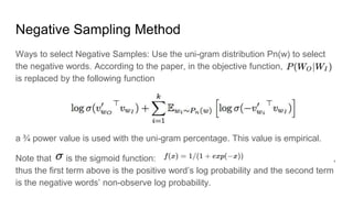
- 14. Negative Sampling Method The principle is that each sample adjusts only a small part of the parametres. The idea is selecting a few negative samples (those which are not around the input centered word) and only updating the output layer weight of the selected negative words and the positive word. Remark: - ItˇŻs a similar way to dropout layer in deep neural network, yet the dropout layer is between the hidden layers, instead of removing the output units. - In the hidden layer, the number of updated weights are not changed -- only the feature weights of input words are to be changed.
- 15. Negative Sampling Method Ways to select Negative Samples: Use the uni-gram distribution Pn(w) to select the negative words. According to the paper, in the objective function, is replaced by the following function a ? power value is used with the uni-gram percentage. This value is empirical. Note that is the sigmoid function: , thus the first term above is the positive wordˇŻs log probability and the second term is the negative wordsˇŻ non-observe log probability.
- 16. Part 1 - Sub-Sampling Method
- 17. Subsampling Heuristic Sub-sampling is important because some words are much more frequent than others. Therefore when the sampling window size is large enough, some words appear quite often in sampling windows yet doesnˇŻt reflect any information (the same goes for a variable with probability 1 doesnˇŻt give any information as entropy). Heuristically, by removing the appearing rate of the same word while conserving the ranking in the whole documents will even improve the final results. The method used in this paper is a sub-sampling by a probability of saving which is of the order . The discard Probability : , t is called the subsampling rate, and f(w) is the frequency of the word w in the corpus.
- 18. Part 2 - Learning Phrase
- 19. Use Phrases Another important contribution is to use the phrases (or word pairs) rather than the words in their training samples. Though this can be regarded as a prepared step, itˇŻs of great importance, given that: - The samples volume is greatly reduced. - The meaning of compositioned phrases are saved. The scores for co-appearance are calculated simply by 2-gram / 1-gram. When the score is large enough, two words are combined into one single phrase. The whole training data set is passing 3-4 times this preprocessing algorithm. In the paper, the obtained phrasesˇŻ vector quality is tested by another analogical reasoning task (72% accuracy).
- 20. Part 3 - Empirical Results
- 21. Analogical Reasoning Task An example for analogical reasoning is as left. Given three phrases, to how much degree can the fourth phrase be inferred from the first three phrase- vectors. By using cosine distance between the vectors, the closest answer is selected and compared with the true answer. This test method is used also in [1]. Figure 3. Examples for Analogical Reasoning test : In each cell, given the first three words, test the accuracy of calculating the fourth.
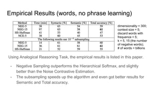
- 22. Empirical Results (words, no phrase learning) Using Analogical Reasoning Task, the empirical results is listed in this paper. - Negative Sampling outperforms the Hierarchical Softmax, and slightly better than the Noise Contrastive Estimation. - The subsampling speeds up the algorithm and even got better results for Semantic and Total accuracy. dimensionality = 300; context size = 5; discard words with frequence < 5; k = 5, 15 (the number of negative words); # of words = billions
- 23. Empirical Results (using phrases) Using Analogical Reasoning Task, the empirical results is listed in this paper. - Using subsampling, Hierarchical Softmax outperforms the other methods ! Yet when no subsampling, HS got the worst accuracy. - As using phrases largely reduced the total number training samples, more training data is needed (to be continued...) dimensionality = 300; context size = 5; discard words with frequence < 5; k = 5, 15 (the number of negative words);
- 24. Empirical Results (using phrases) The paper claims that when using 33 billion words, dimensionality = 1000, and the entire sentence as context size, this resulted in an accuracy of 72%. The best performed model is still HS + subsampling.
- 25. Part 4 - Additive Compositionality
- 26. Additive Compositionality Additive Compositionality is an interesting property of word vector. It shows that a non-obvious degree of language understanding can be obtained by using basic operations (sum here) on the word representation. That is something more than analogical reasoning. The author gave an intuitive explanation as follows (the product of distributions.)
- 28. Conclusion This paper mainly has three contributions: - Using common word pairs (phrase representations) to replace words in the training model. - Subsampling the frequent words to largely decrease training time and get better performance for infrequent words. - Proposing Negative Sampling - Comparing different methodsˇŻ combination and trained a best model (up-to- then) on a huge (30 billions words) data set. - Addressing the additive compositionality of word vector. The works of this paper can be further used in CBOW in [1], and the code is given at https://code.google.com/archive/p/word2vec/
- 29. Referrence [1] Tomas Mikolov, Kai Chen, Greg Corrado, and Jeffrey Dean. Efficient estimation of word representations in vector space. ICLR Workshop, 2013. [2] Frederic Morin and Yoshua Bengio. Hierarchical probabilistic neural network language model. In Pro- ceedings of the international workshop on artificial intelligence and statistics, pages 246¨C252, 2005. [3] Andriy Mnih and Geoffrey E Hinton. A scalable hierarchical distributed language model. Advances in neural information processing systems, 21:1081¨C1088, 2009. [4] Michael U Gutmann and Aapo Hyva ?rinen. Noise-contrastive estimation of unnormalized statistical mod- els, with applications to natural image statistics. The Journal of Machine Learning Research, 13:307¨C361, 2012.


![Background
This paper follows the paper [1] Efficient estimation of word representations in
vector space in 2013.
This paper proposed some important improvements for the Skip-gram model,
which is widely used for obtaining the famous ˇ°word vectorsˇ±. [1] proposed the
CBOW (Continuous Bag-of-words Model) and Skip-gram, using a 3-layer neural
network to train the word-vectors.
While CBOW is entering the context to predict the center, Skip-gram is entering
the center word to predict the context.](https://image.slidesharecdn.com/summarydistributedrepresentationswordsphrases-180308235944/85/Summary-distributed-representations_words_phrases-3-320.jpg)


![In order to reduce the complexity of calculating the weights of output layer.
Hierarchical Softmax (HS) was used in the Skip-gram model. HS was firstly
proposed by [2] Morin and Bengio (2005).
We will introduce the data structure used in HS: Huffman Tree / Coding. Huffman
tree assigns short codes (path) to the most frequent words, and thus the random
walk on the tree will find these words quickly.
The Hierarchical Softmax](https://image.slidesharecdn.com/summarydistributedrepresentationswordsphrases-180308235944/85/Summary-distributed-representations_words_phrases-9-320.jpg)


![The number of parameters rest the same yet a binary Huffman Tree reduced the
computation volume to an acceptable level.
Different methods for constructing the tree structure can be found by [3] Mnih and
Hinton (2009).
HS was proposed in paper [1] a priori and the performance is not satisfying. This
paper compared the results of Hierarchical Softmax with Negative Sampling, and
also Noise Contrastive Estimation - NCE proposed by [4] Gutmann and
Hyvarinen (2012), together with the subsampling trick and using phrase as
training samples.
Huffman Tree](https://image.slidesharecdn.com/summarydistributedrepresentationswordsphrases-180308235944/85/Summary-distributed-representations_words_phrases-12-320.jpg)


![Analogical Reasoning Task
An example for analogical reasoning is
as left. Given three phrases, to how
much degree can the fourth phrase be
inferred from the first three phrase-
vectors. By using cosine distance
between the vectors, the closest answer
is selected and compared with the true
answer.
This test method is used also in [1].
Figure 3. Examples for Analogical Reasoning test : In
each cell, given the first three words, test the accuracy
of calculating the fourth.](https://image.slidesharecdn.com/summarydistributedrepresentationswordsphrases-180308235944/85/Summary-distributed-representations_words_phrases-21-320.jpg)


![Conclusion
This paper mainly has three contributions:
- Using common word pairs (phrase representations) to replace words in the
training model.
- Subsampling the frequent words to largely decrease training time and get
better performance for infrequent words.
- Proposing Negative Sampling
- Comparing different methodsˇŻ combination and trained a best model (up-to-
then) on a huge (30 billions words) data set.
- Addressing the additive compositionality of word vector.
The works of this paper can be further used in CBOW in [1], and the code is given
at https://code.google.com/archive/p/word2vec/](https://image.slidesharecdn.com/summarydistributedrepresentationswordsphrases-180308235944/85/Summary-distributed-representations_words_phrases-28-320.jpg)
![Referrence
[1] Tomas Mikolov, Kai Chen, Greg Corrado, and Jeffrey Dean. Efficient estimation of word
representations in vector space. ICLR Workshop, 2013.
[2] Frederic Morin and Yoshua Bengio. Hierarchical probabilistic neural network language model. In Pro-
ceedings of the international workshop on artificial intelligence and statistics, pages 246¨C252, 2005.
[3] Andriy Mnih and Geoffrey E Hinton. A scalable hierarchical distributed language model. Advances in
neural information processing systems, 21:1081¨C1088, 2009.
[4] Michael U Gutmann and Aapo Hyva ?rinen. Noise-contrastive estimation of unnormalized statistical
mod- els, with applications to natural image statistics. The Journal of Machine Learning Research,
13:307¨C361, 2012.](https://image.slidesharecdn.com/summarydistributedrepresentationswordsphrases-180308235944/85/Summary-distributed-representations_words_phrases-29-320.jpg)