Teknik Pengkodean (2).pptx
- 1. T e k n i k P e n g k o d e a n
- 4. Himpunan event an probabilitas
- 9. Main Compression Techniques and Compression performance âĒ Data compression is often called coding due to the fact that its aim is to find a specific short (or shorter) way of representing data. âĒ Encoding and decoding are used to mean compression and decompression respectively. âĒ We outline some major compression algorithms below: 1. Run-length coding 2. Quantisation 3. Statistical coding 4. Dictionary-based coding 5. Transform-based coding 6. Motion prediction.
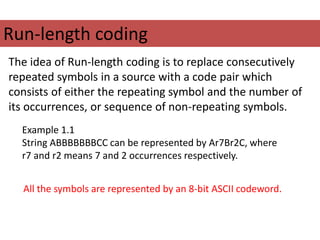
- 10. Run-length coding The idea of Run-length coding is to replace consecutively repeated symbols in a source with a code pair which consists of either the repeating symbol and the number of its occurrences, or sequence of non-repeating symbols. Example 1.1 String ABBBBBBBCC can be represented by Ar7Br2C, where r7 and r2 means 7 and 2 occurrences respectively. All the symbols are represented by an 8-bit ASCII codeword.
- 13. The basic idea of quantisation is to apply a certain computation to a set of data in order to achieve an approximation in a simpler form. Quantisation Example 1.2 Consider storing a set of integers (7, 223, 15, 28, 64, 37, 145). Let x be an integer in the set. We have 7 âĪ x âĪ 223. Since 0 < x < 255 and 2 8 = 256, it needs 8 binary bits to represent each integer above. However, if we use a multiple, say 16, as a common divider to apply to each integer and round its value to the nearest integer, the above set becomes (0, 14, 1, 2, 4, 2, 9) after applying the computation x div 16. Now each integer can be stored in 4 bits, since the maximum number 14 is less than 2
- 15. Example 1.3 We can code the more frequently occurring symbols with fewer bits. The statistical information can be obtained by simply counting the frequency of each character in a file. Alternatively, we can simply use the probability of each character. Statistical coding The idea of statistical coding is to use statistical information to replace a fixed-size code of symbols by a, hopefully, shorter variable-sized code.
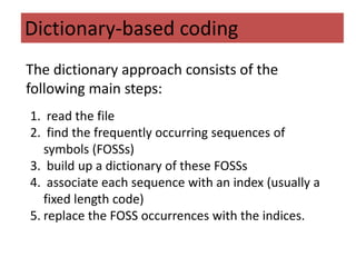
- 16. The dictionary approach consists of the following main steps: Dictionary-based coding 1. read the file 2. find the frequently occurring sequences of symbols (FOSSs) 3. build up a dictionary of these FOSSs 4. associate each sequence with an index (usually a fixed length code) 5. replace the FOSS occurrences with the indices.
- 17. âĒ The transform-based approach models data by mathematical functions, usually by periodic functions such as cos(x) and applies mathematical rules to primarily diffuse data. âĒ The idea is to change a mathematical quantity such as a sequence of numbers to another form with useful features. âĒ It is used mainly in lossy compression algorithms involving the following activities: âĒ analysing the signal (sound, picture etc.) âĒ decomposing it into frequency components âĒ making use of the limitations of human perception. Transform-based coding
- 18. âĒ Motion prediction techniques are lossy compression for sound and moving images. âĒ Here we replace objects (say, an 8 Ã8 block of pixels) in frames with references to the same object (at a slightly different position) in the previous frame. Motion Prediction
- 20. âĒ In this course, we view data compression as algorithmic problems. âĒ We are mainly interested in compression algorithms for various types of data. âĒ There are two classes of compression problems of interest (Davisson and Gray 1976): âĒ Distortion-rate problem Given a constraint on transmitted data rate or storage capacity, the problem is to compress the source at, or below, this rate but at the highest fidelity possible. Compression in areas of voice mail, digital cellular mobile radio and video conferencing are examples of the distortion-rate problems. âĒ Rate-distortion problem Given the requirement to achieve a certain pre-specified fidelity, the problem is to meet the requirements with as few bits per second as possible. Compression in areas of CD-quality audio and motion-picture-quality video are examples of rate-distortion problems. Compression problems
- 21. âĒ In areas of data compression studies, we essentially need to analyse the characteristics of the data to be compressed and hope to deduce some patterns in order to achieve a compact representation. âĒ This gives rise to a variety of data modelling and representation techniques, which are at the heart of compression techniques. âĒ Therefore, there is no âone size fits allâ solution for data compression problems. Algorithmic solutions
- 22. âĒ Due to the nature of data compression, any compression algorithm will not work unless a decompression approach is also provided. âĒ We may use the term compression algorithm to actually mean both compression algorithm and the decompression algorithm. âĒ In this subject, we sometimes do not discuss the decompression algorithm when the decompression process is obvious or can be easily derived from the compression process. However, you should always make sure that you know the decompression solutions. âĒ In many cases, the efficiency of the decompression algorithm is of more concern than that of the compression algorithm. âĒ For example, movies, photos, and audio data are often compressed once by the artist and then decompressed many times by millions of viewers. âĒ However, the efficiency of compression is sometimes more important. For example, programs may record audio or video files directly to computer storage. Compression and decompression
- 23. âĒ The performance of a compression algorithm can be measured by various criteria. It depends on what is our priority concern. In this subject guide, we are mainly concerned with the effect that a compression makes (i.e. the difference in size of the input file before the compression and the size of the output after the compression). âĒ It is difficult to measure the performance of a compression algorithm in general because its compression behaviour depends much on whether the data contains the right patterns that the algorithm looks for. âĒ The easiest way to measure the effect of a compression is to use the compression ratio. âĒ There are several ways of measuring the compression effect: âĒ Compression ratio. This is simply the ratio of size.after.compression to size.before.compression or Compression ratio = size.after.compression size.before.compression âĒ Compression factor. This is the reverse of compression ratio. Compression factor = size.before.compression size.after.compression âĒ Saving percentage. This shows the shrinkage as a percentage. Saving percentage = size.before.compression â size.after.compression size.before.compression % Note: some books (e.g. Sayood(2000)) defines the compression ratio as our compression factor. Compression performance
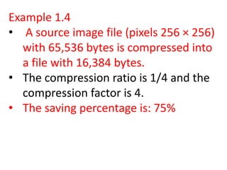
- 24. Example 1.4 âĒ A source image file (pixels 256 Ã 256) with 65,536 bytes is compressed into a file with 16,384 bytes. âĒ The compression ratio is 1/4 and the compression factor is 4. âĒ The saving percentage is: 75%
